ISSN: 0970-938X (Print) | 0976-1683 (Electronic)
Biomedical Research
An International Journal of Medical Sciences
Research Article - Biomedical Research (2017) Volume 28, Issue 16
A hybrid segmentation approach for detection and classification of skin cancer
Vellore Institute of Technology, Vellore, Tamil Nadu, India
Accepted date: June 2, 2017
Advancement in Computer Aided Diagnostic system (CAD) enhances the detection and classification of domain experts and reduces the time rapidly for them. The CAD systems can be used in hospitals as an alternate method. The objective of the paper is to present the effectiveness of the detection and classification of skin cancer. The proposed methodology concentrates on comparing the median filter and Adaptive Median Filter (AMF) and suggesting on one, the segmentation can be done by a hybrid approach where the marker controlled watershed algorithm is fused with the active contour algorithm, the feature extraction is done with the help of basic statistical methods and the Grey Level Co- Occurrence Matrix (GLCM) with the Support Vector Machine (SVM) for classification. SVM is used to classify the input as cancerous or not. The experiment is carried out on 250 images consists of 100 normal images and 150 abnormal images (benign and melanoma images) from a skin dataset. The classification accuracy shows 94% after the classification.
Keywords
Adaptive median filter, Active contour, Marker control watershed, Grey level co-occurrence matrix (GLCM), Support vector machine (SVM).
Introduction
The computer aided diagnostic system is something which helps in the experts to process the system pretty quickly. The CAD system helps in assisting the physician to make decision so it helps in decision support system. The analysis can be done in a very short time using CAD systems. CAD systems are built in such a way that they can detect a melanoma image. Cancer is a dreadful disease that occurs most commonly nowadays. It can be treated but still the treatment is a very challenging one. The dreadful disease can occur any time right from kids to grown up. We are discussing on the various possibility to detect the tumour earlier. Skin cancer can be of various types where melanoma is a life threatening disease. The melanoma and benign are two classes where melanoma meaning the cancerous one and the other one is not. Skin cancer can have various stages. It can occur from a mole, exposure to sunlight and hereditary as well. This proposed method can be using the adaptive median filter and the comparison on the adaptive and median filter are also expressed. The segmentation can be a hybrid method followed by a feature extraction and then finally the classification procedure to determine the accuracy.
Related Work
There are various filtering techniques discussed on skin cancer detection like image scaling, color space transformation [1] and the hair removal algorithm of dull razor software can also be included [2] that removes the hair in an image. The contrast enhancement can also apply as a filter [3] which helps in improving the contrast. Finding the region of interest is a very important role to play with. And it can be using Gradient Vector Flow (GVF), level set methods, adaptive thresholding, adaptive snake, EM level set, [4] Fuzzy based split and merge. One another segmentation which helps in maximum entropy threshold. The watershed algorithm which is used mostly for segmentation is explained in [5,6]. The feature extraction can explain on GLCM, [7] ABCD features [8-11]. Gabor filters and the other methods to extract the features explained [12-16]. The extracted features are subjected to classification. The accuracy plays a vital role in medical image processing. The accuracy obtained are calculated based on the various metrics of classification from algorithms like artificial neural networks [17,18] support vector machine, K-nearest neighbour [19,20] and the back propagation algorithm.
This paper is organised as follows: section 2 presents the related works and section 3 explains the proposed methodology describing the pre-processing of skin cancer images, the hybrid segmentation methodology, the feature extraction on the segmented image and finally the classification done by four different classifiers. Section 4 describes the performance evaluation and section 5 explains the obtained results that are found by the above steps. And finally section 6 draws a conclusion and gives a hint for the future work to be done.
Materials and Methods
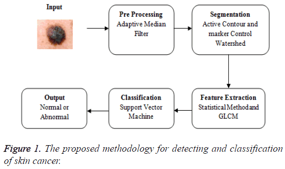
The proposed methodology in Figure 1 explains the overview of the skin cancer detection and classification. The input image is taken and that is subjected to the pre-processing phase. Preprocessing is removing the noise. The medical imaging works well for the noise free images. The pre-processing uses the adaptive median filter to remove the noise. Then the median filter and the adaptive median filter are compared and the values based on the metrics are calculated. The various metrics are compared for both the median filter and the adaptive median filter. The adaptive median filtered image is fed as an input to the segmentation phase. The segmentation uses the hybrid method of both the active contour and the marker control watershed algorithm. The segmentation using active contour is extracted and the output of that is fed as an input to marker control watershed algorithm. Now the segmented image is extracted for GLCM features and the basic statistical method. Then the features are fed as an input to the support vector machine to examine the accuracy.
Image enhancement
The first step is to acquire an image. The acquired image is then subjected to pre-processing. Pre-processing is the step which is used to enhance an image. The enhancement stage is used to filter the noise and brighten the image. The error rate gets reduced and the pixel intensities are improved by using the noise filters. There are various noise filters like box filter, weighted average filter, median filter, mean filter, mode filter and various other filters. Our proposed method uses the median filter and the adaptive median filter for pre-processing and the comparative results are discussed here.
Median filter
Median filter is one of the best used filters for pre-processing medical images. The median filter is a filter which helps to remove noise and brighten the image without noise factor. The median filter operations can be by using masks. Firstly the image is arranged in ascending order and then the median of the image is found and replaced by the original pixel intensity values.
Adaptive median filter
The adaptive median filter is an advanced version of median filter. The adaptive median filter as the name suggests uses the adaptive mask which differs from application to application. The adaptive median filter uses the following algorithm.
Stage 1:
H1=Fmedian-Fmin
H2=Fmedian-Fmax
If F1>0 and F2<0 go to stage 2
Else increase the filter size
If filter size = Smax repeat stage 1
Else output Fmedian
Stage 2:
G1=Fxy-Fmin
G2=Fxy-Fmax
If G1>0 and G2<0, display Fxy
Else display Fmedian
Sxy is the support of the filter centered at x, y.
Fmedian is nothing but the median of gray levels at Sxy. Fmin is the minimum gray level at Sxy
Fmax, Fmin are the minimum and the maximum gray levels at Sxy.
Fxy is simply the gray level at coordinates x, y.
Smax is the maximum size allowed size of Sxy.
The adaptive median filter algorithm discusses about 2 stages in stage 1 the mask is first determined adaptively. Then the difference of median and the minimum gray level value is found. Then the difference of median and the maximum gray level value is found and they are compared, if the former is greater than zero and the latter is lesser than zero go to stage 2. There the difference between the centre pixel and the minimum intensity level pixel is found and then the difference between the centre pixel and the maximum intensity pixel is found and then if the former is greater than zero and the latter is less than zero the value at Fxy is assumed as the final value. Else the size of the mask is increased if the mask is less then repeats the stage 1 else replace the value with the median of the mask.
Comparison of median filter and the adaptive median filter
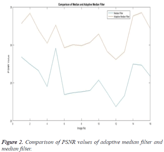
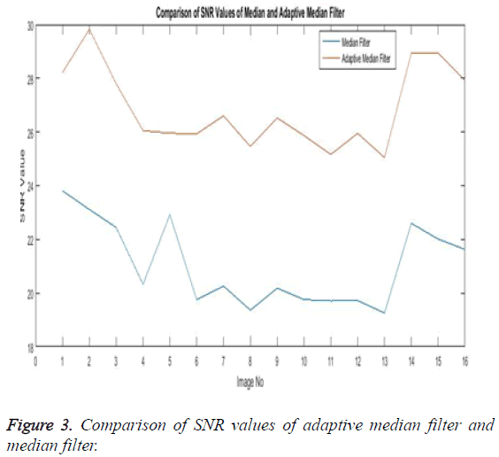
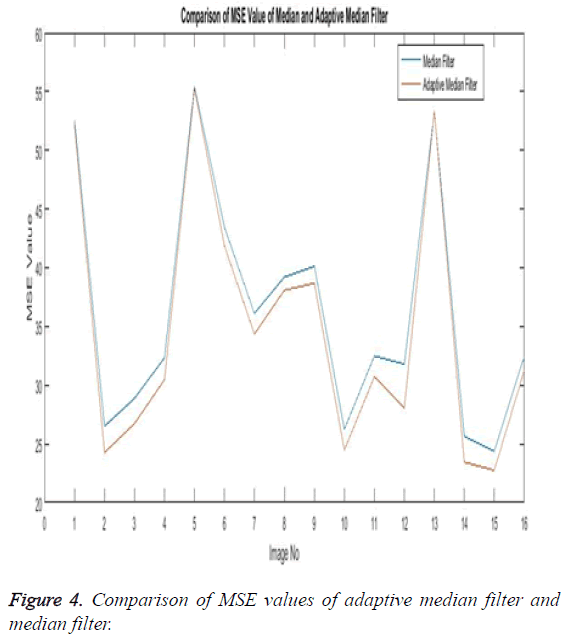
The median filter and the adaptive median filter are good at their own performance. We have tested with the dataset that we have on both the median filter and the adaptive median filter. The adaptive median filter has given a better result when compared to that of a median filter as far as our dataset is concerned. The adaptive median filter and the median filter are tested with 75 images. The samples of the tested images are displayed in Table 1. The comparative study of the filters can be represented by means of a graph as well. The adaptive median filter therefore is used to remove the noise and enhance the image.
| Adaptive median filter | Median filter | |||||
|---|---|---|---|---|---|---|
| Input Image | PSNR | SNR | MSE | PSNR | SNR | MSE |
| 1 | 32.8177 | 28.2152 | 52.1294 | 28.411 | 23.8085 | 52.54 |
| 2 | 34.169 | 29.8256 | 24.2677 | 27.4568 | 23.1133 | 26.5067 |
| 3 | 31.9478 | 27.7946 | 26.7344 | 26.5975 | 22.4442 | 28.8753 |
| 4 | 30.2266 | 26.05 | 30.4705 | 24.5032 | 20.3266 | 32.3335 |
| 5 | 32.6065 | 25.9556 | 55.2646 | 29.5707 | 22.9198 | 55.4294 |
| 6 | 29.6225 | 25.9313 | 41.8588 | 23.4473 | 19.7562 | 43.4436 |
| 7 | 30.0273 | 26.6006 | 34.3551 | 23.6879 | 20.2613 | 36.1168 |
| 8 | 29.9059 | 25.4595 | 38.0873 | 23.814 | 19.3676 | 39.2061 |
| 9 | 30.329 | 26.522 | 38.6791 | 23.9909 | 20.1839 | 40.121 |
| 10 | 31.44659 | 25.8673 | 24.4702 | 25.3576 | 19.7589 | 26.2431 |
| 11 | 29.1108 | 25.1612 | 30.7278 | 23.658 | 19.7083 | 32.4846 |
| 12 | 28.075 | 25.9492 | 28.0483 | 21.8482 | 19.7224 | 31.7959 |
| 13 | 29.085 | 25.049 | 53.3695 | 23.2945 | 19.2585 | 53.2685 |
| 14 | 33.8174 | 28.9424 | 23.4498 | 27.4732 | 22.5982 | 25.6438 |
| 15 | 34.2554 | 28.9412 | 22.7558 | 27.3259 | 22.0117 | 24.3775 |
| 16 | 32.1612 | 27.9163 | 31.2433 | 25.8704 | 21.6254 | 32.4126 |
Table 1: Comparison of the metrics on pre-processing such as PSNR, SNR and MSE between median filter and adaptive median filter.
Segmentation
The segmentation is the process by which the entire image is divided into multiple parts. The segmentation helps in identifying the region of interest. Here we use the active contour segmentation algorithm and marker control watershed algorithm for the process of segmentation. The pre-processed image is fed into the active contour algorithm as this algorithm supports noise free images, and the output of the active contour is fed as an input to the marker control watershed algorithm. And the features are then extracted from the segmented image.
Active contour
The enhanced image is fed as input to the segmentation phase. There are three important steps in this phase. The first step is to represent object boundary or any parametric curve. The second step focuses on energy calculation and that energy should be minimised. Step three starts at a point and it moves towards a certain boundary and then it shrinks.
The contour point is defined as
C(s)=(A (s), B (s)) → (4)
The energy can be calculated as
Energy=Internal energy+External energy+Constraint energy
The energy is calculated as the sum of internal energy, external energy and constraint energy. Internal energy is of elastic energy and blending energy.
Internal energy=Elastic energy+Blending energy
Elastic energy=1/2 ∫ α (s) mod C(s)2 ds → (5)
Blending energy=1/2 ∫ β (s) mod css2 ds → (6)
By using Equations 4-6 we compute the energy by using the elastic and bending property the elastic property gives a stiff image whereas the blending energy gives a smooth region. Internal energy is obtained by adding elastic energy and blending energy. The next calculation is the external energy or the boundary calculations. They are represented as follows
External energy=∫0 1Image C (s) ds → (7)
The final active contour can be represented as the sum of the internal energy, external energy and the constraint energy as discussed in the above equations.
Marker controlled watershed
The obtained output is fed into the next segmentation phase. The gradient magnitude is computed. The background markers and the foreground objects are detected using the opening followed by the reconstruction phase and then the closing is performed. The watershed ridges are identified. Colored watershed labels are marked and the region of interest is extracted by means of marked watersheds.
Feature extraction
The feature extraction is the next phase of the detection and classification methodology. The features are extracted by the segmented image and then the feature extraction is done by combining the GLCM and normal statistical method.
Normal statistical method
The basic statistical methods are used to calculate the area, mean, variance and standard deviation in the features. The features calculation is tabulated according to the below Equations 1-4. Area is calculated as the whole segmented image. Mean is the whole summed up divided by total and variance and standard deviation is calculated along with the GLCM features extraction.
 → (8)
→ (8)
 → (9)
→ (9)
 → (10)
 → (11)
GLCM
GLCM is a second order feature, it is calculated at a distance d with an angle θ. The input is arranged as its corresponding cooccurrence matrix which has nearly 20 features to be considered the features are entropy, energy, contrast, correlation, homogeneity, cluster prominence, cluster shadowing, dissimilarity, maximum probability, sum of squares, sum average, sum variance, sum entropy, difference variance, difference entropy, etc. The formula that is used to calculate the above features are as listed below.
Homogeneity
They contain the homogenous that is the same gray level values
 → (12)
Contrast
The measure of local intensity variation
 → (13)
Local homogeneity (LH)
Relatively higher value will be obtained out of this feature
 → (14)
Entropy
It is actually representing the disorders
 → (15)
Correlation
The measure of intensity dependence
 → (16)
Sum of square: Variance
It is the average of the mean
 → (17)
Sum average
The sum of average is something where the total value is found.
 → (18)
Sum entropy
The sum entropy is as follows
 → (19)
Difference entropy
The difference entropy is as follows
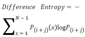 → (20)
Cluster shade
The cluster shade is as follows

Cluster prominence
The cluster prominence is as follows
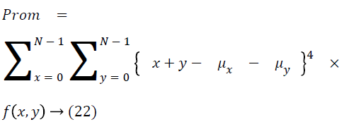
Thus the Equations 4-22 explain how the features can be extracted from the segmented image and how the features can be fed into the classifiers.
Classification
The classification is the final stage which classifies into benign or melanoma image. Benign meaning a normal image and melanoma the cancerous image. Support Vector Machine (SVM) is the classifier used here where it uses the hyper plane to classify and misclassify the classes. Two classes defined one is class 1 the normal one, class 2 the cancerous one. The features are fed into the classifier and the classification accuracy obtained is 94%.
Results and Observations
The results and discussion of the hybrid segmentation algorithm that helps to detect and classify the skin cancer images are discussed in this session. This session explains the result of all the four phases preprocessing, segmentation, feature extraction and classification.
Preprocessing
The noise removal stage or the first phase of any medical image processing is the preprocessing phase. Here the preprocessing phase uses both the median filter and the adaptive median filter and then both are eventually compared. The below Table 1 explains the comparison of both the adaptive median filter and the median filter.
The Table 1 tabulates the value of the metrics of pre-processing such as Peak Signal to Noise Ratio (PSNR), Signal to Noise Ratio (SNR) and Mean Square Error (MSE). The metrics are calculated as follows
 → (1)
→ (1)
 → (2)
→ (2)
k × l-noise free order of a monochrome image I
J-Noisy approximation
Peak signal to noise ratio (PSNR) =20 × log10 (MPV)-10 × log10 (MSE) → (3)
MPV: Maximum Possible Pixel Value
MSE: Mean Square Error
The Equations 1-3 shows how the metrics of pre-processing are calculated based on the equation that is discussed. They can also be expressed in form of a comparison graph.
Thus Figures 2-4 can very well show that the comparisons were made and they evidently show that the adaptive median filter has an upper hand over a median filter. And hence the dataset works well for the adaptive median filter rather than the median filter.
Segmentation
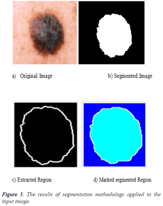
The segmentation can be done for the preprocessed image. The preprocessed image can be fed as an input to the segmentation phase. The segmentation uses the active contour algorithm and the marker control watershed algorithm. The active contour uses three important steps: the first one is to identify the object boundary, the second one is to compute the energy that is the internal energy, external energy and the constraint energy. Then the final object shrinks and the segmented portion is obtained. The output of that is fed as an input to the marker controlled phase. The gradient magnitude is calculated. The foreground image is obtained by opening followed by the reconstruction phase. Then the background values are marked. The watershed transform is used to calculate the ridges and the final result is visualized. The segmentation result is given in Figure 5 after all the segmentation process applied.
Feature extraction
The feature extraction helps to extract the features. There are 27 features extracted from the segmented image. The various features play a very vital role since the features are the essential elements that mostly determine the accuracy in an image. The feature extraction can be called as the heart of the process. The extracted features are then fed to the classification phase so as to classify the class 1 normal and the class 2 melanoma images. The classification and the misclassification are formed by the support vector machine which is described in the below equation and the table.
The Table 2 explains about the various features of an image. And the various features are calculated based on the Equations 5-15 given above. The features are extracted and are fed into the support vector machine.
| Features | Image 1 | Image 2 | Image 3 |
|---|---|---|---|
| Auto correlation | 35.34233 | 27.66175 | 36.37562 |
| Contrast | 1.47595 | 1.843052 | 2.366154 |
| Correlation1 | 0.93896 | 0.923592 | 0.900866 |
| Correlation 2 | 0.23104 | 0.190702 | 0.191454 |
| Cluster prominence | 2383.906 | 2374.833 | 2386.172 |
| Cluster shadowing | -73.4408 | -99.3462 | -43.8361 |
| Dissimilarity | 0.21085 | 0.263293 | 0.338022 |
| Energy | 0.477245 | 0.471532 | 0.466938 |
| Entropy | 0.821636 | 0.845376 | 0.872978 |
| Homogeneity | 0.970481 | 0.963139 | 0.952677 |
| Homogeneity 2 | -0.80345 | -0.76657 | -0.71656 |
| Maximum probability | 0.817476 | 0.806446 | 0.78914 |
| Sum of Squares | 0.973644 | 0.967088 | 0.957747 |
| Sum average | 0.541769 | 0.543364 | 0.556152 |
| Sum variance | 9.795623 | 8.129617 | 10.12416 |
| Sum entropy | 0.800757 | 0.819304 | 0.839507 |
| Difference variance1 | 12.09192 | 12.0602 | 11.9345 |
| Difference variance 2 | 1.431493 | 1.77372 | 2.251894 |
| Difference entropy | -0.12963 | -0.10083 | -0.10106 |
| Informational measure of correlation | 0.060685 | 0.053711 | 0.053772 |
| Informational measure of correlation 2 | 0.99859 | 0.998505 | 0.998512 |
| Maximum correlation coefficient | 0.99869 | 0.99861 | 0.998617 |
| Mean | 0.7609 | 0.4475 | 0.777 |
| Variance | 0.1819 | 0.2472 | 0.1733 |
| Standard deviation | 0.4265 | 0.4972 | 0.4162 |
| Area | 49966.75 | 29358.88 | 50948.88 |
Table 2: The various features of both the GLCM and the basic statistical methods are listed below for three sample images.
Classification
The classification uses the Support Vector Machine (SVM) to predict the classification accuracy. The classification can be expressed by using the hyper plane to classify and misclassify the elements. The weight bias and the input are used to classify the images clearly.
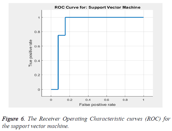
Based on the Equations 16-18 the performance analysis of the proposed methodology is performed. The proposed methodology explains the adaptive median filter for preprocessing followed by a hybrid segmentation method followed by a feature extraction algorithm and finally to a SVM classifier to obtain an accuracy .The Receiver Operating Characteristic curve (ROC) in Figure 6 explains about the feature selection and the classification accuracy which is 94%.
The input image is fed into the enhancement technique using the adaptive median filter. Then the pre-processed image is segmented using the two way segmentation technique which is fed into the feature extraction phase and then is classified using the support vector machine. The values are calculated based on True Positive (TP), True Negative (TN), False Positive (FP) and False Negative (FN).
The accuracy can be calculated from below equation
Accuracy=(TP+TN)/(TP+TN+FP+FN) → (23)
The sensitivity can be calculated from below equation
Sensitivity= TP/(TP+FN) → (24)
The specificity can be calculated from below equation
Specificity=TN/(TN+FP) → (25)
The classification algorithm provides the analyses of 250 images out of which 100 are benign and rest 150 are melanoma images.
The classification accuracy is said to be 94%. Table 3 gives the sensitivity and specificity. Thus the Table 3 gives the values of the accuracy to be 94%, sensitivity to be 86.32% and specificity to be 92.9%. The area under the curve is estimated to be 0.90566 (Table 4).
| Performance measures | Percentage (%) |
|---|---|
| Accuracy | 94 |
| Sensitivity | 86.32 |
| Specificity | 92.9 |
Table 3: Performance evaluation using the support vector machine classification.
| Methods | Accuracy | Dice coefficient | Jaccard index |
|---|---|---|---|
| Otsu’s thresholding | 87.22 | 89.63 | 91.32 |
| Active contour | 92.34 | 90.43 | 90.67 |
| Watershed | 89.43 | 88.63 | 89.93 |
| Marker controlled watershed | 93.56 | 91.54 | 92.83 |
Table 4: Comparison on segmentation algorithms by using various segmentation metrics.
Discussion
Thus the proposed methodology provides an accuracy of 94% and so the error rate remains 6% as far as the medical image processing is concerned the margin of error must be comparatively less so the future work focuses on how to improve the accuracy by increasing the dataset and also the concentration may be put in much on the feature extraction that can also extract much more features that could improve the accuracy as well.
The data set can be increased and the features can also be improved to give good classification accuracy rate.
References
- Kostopoulos S. An ensemble template matching and content-based image retrieval scheme towards early stage detection of melanoma. Image Anal Stereol 2016; 35: 137-148.
- Ali AH, Enass HH, Alaa N. Analysis and classification of kidney images using watershed segmentation and texture properties. IJCSMC 2016; 5: 592-604.
- Jamil U. Computer based melanocytic and nevus image enhancement and segmentation. Biomed Res Int 2016; 1-14.
- Singh A, Priyanka R, Ritesh M. Melanoma detection using local classes of histogram of equivalence pattern. Int J Comp Sci Info Secur 2016; 14: 415-430.
- Antony A, Arun R, Asha S, Betsy M, Tessy AV. Skin cancer detection using artificial neural networking. Skin 2016; 4.
- Kavimathi P. Comparative analyses of classifiers for diagnosis of skin cancer using dermoscopic images. Ind J Sci Technol 2016; 9.
- Agaian S, Monica M, Anthony TC. A new acute leukemia-automated classification system. Comp Meth Biomech Biomed Eng Imaging Visual 2016; 1-12.
- Sasikala M, Kumaravel N. Comparison of feature selection techniques for detection of malignant tumor in brain images. International Conference of IEEE India Council (INDICON 05) 2005; 212-215.
- Liu H, Yu L. Toward integrating feature selection algorithms for classification and clustering. IEEE Trans Knowledge Data Eng 2005; 17: 491-502.
- Jerant AF, Johnson JT, Sheridan CD, Caffrey TJ. Early detection and treatment of skin cancer. Am Family Phys 2000; 62: 381-382.
- Nachbar F, Stolz W, Merkle T. The ABCD rule of dermatoscopy. J Am Acad Dermatol 1994; 30: 551-559.
- Gogoi UR. A study and analysis of hybrid intelligent techniques for breast cancer detection using breast thermograms. Hybrid Soft Computing Approaches. Springer India 2016; 329-359.
- Masood A. Developing improved algorithms for detection and analysis of skin cancer. Diss 2016.
- Verma A, Gayatri K. A survey on digital image processing techniques for tumor detection. Ind J Sci Technol 2016; 9: 1-15.
- Azadeh NH, Adel A, Afsaneh NH. Comparing the performance of various filters on skin cancer images. International Conference on Robot PRIDE 2013-2014-Medical and Rehabilitation Robotics and Instrumentation 2013-2014 Procedia. Computer Science 2014; 42: 32-37.
- Abdul JJ, Sibi S, Aswin RB. Artificial neural network based detection of skin cancer. Int J Adv Res Electr Electron Instr Eng 2012; 1: 200-205.
- Mariam A, Mai SM, Amr S. Automatie detection of melanoma skin cancer using texture analysis. Int J Comp Appl 2012; 42.
- Silveira M, Nascimento JC, Marques JS. Comparison of segmentation methods for melanoma diagnosis in dermoscopy images. IEEE J Signal Proc 2009; 3: 35-45.
- Chiem A, Al-Jumaily A, Khushaba RN. A novel hybrid system for skin lesion detection. Proceedings of the 3rd International Conference on Intelligent Sensors, Sensor Networks and Information Processing 2007; 567-572.
- Emre Celebi M, Hassan AK, Bakhtiyar U. A methodological approach to the classification of dermoscopy images. Comp Med Imag Graph 2007; 31: 362-373.
