ISSN: 0970-938X (Print) | 0976-1683 (Electronic)
Biomedical Research
An International Journal of Medical Sciences
Research Article - Biomedical Research (2017) Volume 28, Issue 10
Classification of mammograms for breast cancer detection based on curvelet transform and multi-layer perceptron
In this paper, classification of mammograms for breast cancer detection based on Discrete Curvelet Transform (DCT) and Multi-Layer Perceptron (MLP) is proposed. The mammogram patches are first filtered by Column wise neighborhood operations Filter (COLFILT). Enhanced patches are further decomposed into four sub-bands by using DCT. Dense Scale Invariant Feature Transform (DSIFT) method is use to extract the six rotation and scale invariant features for all the sub-bands. By using these sub-bands of all the patches, a feature matrix is created that is further processed by MLP for classification. The proposed method is tested using the Image Retrieval in Medical Application (IRMA) dataset. Numerical validation results and graph shows the significance of proposed scheme as compared to state of art existing schemes.
Keywords
Mammography, Detection, Support vector machine, Multi-Layer perceptron
Introduction
The American Cancer Society (ACS) recommends that every woman aged 40 or above should have a mammogram test every year and calls it a gold standard for breast cancer detection. Early detection of breast cancer plays a significant role for high survival rate to a great extent. Breast cancer is recognized as the second most fatal type of cancer in women. Various algorithms have been developed for mammography analysis to obtain better classification efficiency, robustness and accuracy. The three class classification is still an open research area due to the fact that tumour type can be normal, benign or malignant. Breast cancer usually takes time to develop and its symptom appears very late. As there is no effective way to cure later stage breast cancer, early detection of breast cancer increases treatment options and patients' survivability [1]. Therefore for the early detection of breast cancer it is recommended by America Cancer Society (ACS) that every woman who has risk factor of breast cancer should take screening test once in a year [2].
Abirami [3] used wavelet features for the two class classification of digital mammograms, they have achieved 93% accuracy, and however the dataset is small. Jasmine et al. [4] performed two class classification with his proposed method based on wavelet analysis using ANN. This experiment is performed using MIAS database of 322 images and has achieved accuracy up to 87%. Li et al. [5] presents mass classification in mammograms based on two concentric masks and discriminating texton. They have achieved accuracy up to 86.92% by using small dataset of 130 mammogram images. Mazurowski et al. [6] proposed a template based a recognition algorithm for breast masses. Their data set is based of 1,852 Digital Database for Screening Mammography (DDSM) images and achieved accuracy up to 83%. Casti et al. [7] presents three class classification using contour independent detection. This method was tested on a total of 2105 mammogram images but the accuracy rate was not so promising. Elter and Hasslmer [8] performed classification using Artificial Neural Network (ANN) and Euclidean metric classifier respectively and achieved a performance over 85%. Tao et al. [9] compare the performance of two classifier named curvature scale space, and local linear embedded matric using a database of 476 and 415, and the accuracy of the two classifiers are 75% and 80% respectively. Muhammad et al. used fusion of discrete cosine transform and discrete wavelet transform features to classify mammograms in 3 classes [10], they used data in the MIAS database of 322 images and obtained high accuracy of 96.97% and 98.39% respectively.
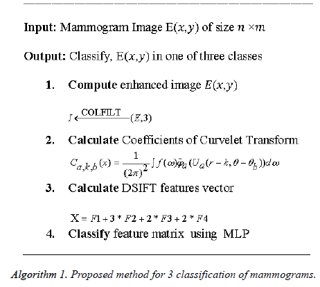
Many researchers have used curvelet transform in the medical images. Lin et al. [11] used curvelet transform for the detection of prostate cancer. Eltoukhy et al. [12] used curvelet transform for breast cancer diagnosis, they used 122 images of MIAS and achieved accuracy of 98.59%. Ucar et al. [13] used DCT in extreme learning for the facial detection. Kiran et al. [14] also used DCT and DWT to analysis the microclassification of mammogram images, they have used 230 MIAS database images and achieved accuracy 93.86 % and 90.43% respectively. ANN has been widely used for the classification of biomedical images. ANN is capable of improving accuracy for classification specific biomedical problems [15]. Standard MLP use back propagation algorithm which train feed forward ANN (Algorithm 1). They need training as they are supervised networks.
From literature, it can be seen that significant results are achieved for two class (normal vs. abnormal) classification. But for three class (normal benign malignant) classification either data set is small or it has not achieved very promising results. In this work, novel three class classification technique for large dataset of mammograms using MLP is proposed. A flow chart of the proposed method is given in Figure 1.
The rest of the paper is organized as: Section 2 related to the feature extraction and representation. Section 3 presents the results and discussion and section 4 comprises the conclusion.
Proposed Scheme
Let E be an input image having dimensions M × N.
Enhancement technique is use to enhance the possibly degraded contrast in some of mammogram images, therefore as pre-processing step we have applied a contrast enhancement technique i.e.

Where COLFILT filter enhances the image E depending upon the global mean and global variance of the image [16]. Figure 2 presents the original and enhanced image.
Two-discrete curvelet transform
In next step enhanced mammogram patch I is decomposed into four sub-bands coefficients by using Discrete Curvelet Transform (DCT). DCT is an image representation technique used in computer vision. It was proposed by Candes and Donoh [17]. DCT codes image edges more efficiently than wavelet transform [18] and it has useful geometric features that can be used as a feature vector in medical image processing. Eltoukhy et al. [19] has used DCT for the mammogram images.
Let L be a function that has a discontinuity across a curve and is smooth otherwise, and consider approximating L from the best n-terms in the expansion. The squared error of such an nterm expansion obeys [20].

Where Lf is the approximation from n best Fourier coefficients. Equation 3 shows expansion for wavelet,

Where Lw is the approximation from n best wavelet coefficients. Equation 4 shows expansion for curvelet expansion.

Where Lc is the approximation from the n best curvelet coefficients. The Equation 4 also shows that the MSE will be reduced in DCT.
A fast DCT [21] has a two dimensions space R2 with ω as the frequency domain variable and x as the spatial variable. r and θ are the polar coordinates in the frequency domain. A pair of windows V(t) and W(r) are defined, which will be called the angular window and the radial window respectively. The V is taking real arguments and supported on r ((-1, 1) and the W is taking positive real arguments and supported on r (1/2, 2).


For each a ≥ a0, a frequency window Ua is define as

The scaled and shifted curvelet in frequency domain is defined as:

From, Plancherel’s theorem, curvelet coefficients can be computed as:

Ca,k,b (x) are curvelet coefficients in 4 sub-bands of spatial frequencies namely F1, F2, F3 and F4.
Dense scale invariant feature transform
In next step DSIFT descriptor is extracted to all the sub-bands components. Dense SIFT scale-space extrema detection used Difference-of-Gaussian (DOG) function to identify potential interest points [22], which were invariant to scale and orientation.

Where α is a constant multiplicative factor and G (x, y, σ) represent variable scale Gaussian i.e.

Equation 11 can be written as:

Where scale space of an image L(x, y, σα) is the convolution of G with an input image I (x, y). DOG is used here instead of Gaussian to improve the computation speed.
The DSIFT descriptor is applied to all the sub-bands with step size 4 and radius size 5, feature matrices having dimension (128 × 400) are extracted for all the sub-bands. From the columns of this matrix six time domain features kurtosis, mean, skewness, energy, maximum and standard deviation are extracted for each sub-band. The resultant feature matrix is of the shape of (128 × 6) that reshaped into a vector form of (1 × 768). Multiplicative coefficient is applied to the sub-band images according to the Equation 13.

Equal zero padding is perform on the start and end columns such that x as (1 × 784). Enhancement and feature extraction steps are perform on all the data set so that we have a data matrix Y of the shape (2296 × 785), where 2296 is the number of the sample images and 784 is the number of features of the each sample. Every sample has a last column label belongs to its receptive patch class.
Multi-layer perceptron
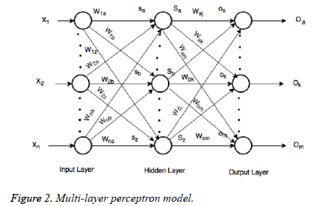
In the last step features set Y is used as input to ANN. They are mostly used in classification due to significant success in nonlinear mapping among the input features and desired output. MLP is a ANN consist of an input layer, an output layer and hidden layer. The number of hidden layers depends upon the designer and application. Each node in MLP performs two functions. At first step it computes the weighted sum of the input along with the bias.

Where Xi shows the ith input, Wij indicates the connection weight from input i to jth hidden layer, θj is bias of jth hidden layer and n is number of input neuron.
Activated function is use as to generate the output of each neuron, i.e.

f (sj)=sigmoid (sj) and is defined as:

The final output is defined as:

Where Wjl indicates the connection weight from jth hidden layer to output l, is bias of lth hidden layer and l is the output neuron. In output layer each neuron use activated function to generate the output, i.e.

Where f (ol)=sigmoid (ol) and is defined as:

In the last step features set Y is used as input to MLP to classify this data set into three classes. To train the MLP optimal values of weights and bias are required for desirable output. In our experiment we have used MLP with 500 hidden units and one hidden layer. Figure 2 presents the basic concept of MLP.
Results and Discussion
We have used IRMA dataset [22] for the evaluation of proposed technique. A total of 2796 patches of original mammogram images are used for this experiment.
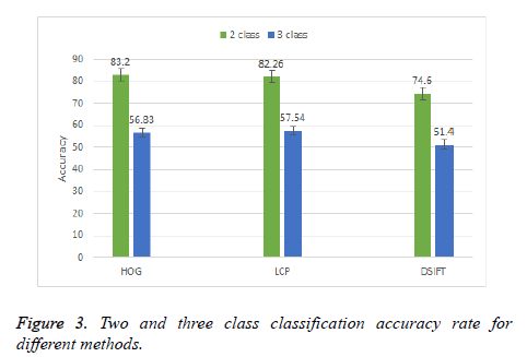
Initially a two and three class classification is done by using DSIFT, Local Configuration Pattern (LCP) and Histogram Oriented Gradient (HOG) methods. Figure 3 shows the result of two and three class classification. It can be observed that in two class classification HOG method perform better with accuracy rate 83.2%. The other two schemes LCP and DSIFT has accuracy rate 82.26% and 74.6% respectively. In three class classification HOG method performs better than the other two schemes but the results is not so promising, with the best result accuracy of 56.83%. SVM with linear kernel is used for both the classifications.
Table 1 presents the validity assessment measures of existing schemes for two class classification. In all assessment measures HOG shows better performance than other two methods except the sensitivity, where it has slightly less value than LCP. LCP performs better than DSIFT in all five validity assessment measure, it can easily be seen in the quantitative comparison table that HOG method performs better than other two methods.
| HOG | LCP | DSIFT | |
|---|---|---|---|
| PPV | 0.842 | 0.841 | 0.681 |
| NPV | 0.916 | 0.898 | 0.862 |
| Sensitivity | 0.863 | 0.871 | 0.851 |
| Specificity | 0.821 | 0.786 | 0.712 |
| MCC | 0.813 | 0.811 | 0.699 |
| ROC | 0.833 | 0.819 | 0.714 |
Table 1. Validity assessment measures for two classes.
Similarly, Table 2 shows the quantitative comparison for three class classification of existing and proposed schemes. The same assessment measures, as given in Table 1, have been used to test the performance of different methods for three class classification. Among existing three methods LCP outperforms all assessment measures except sensitivity, whereas HOG method has the better result with 0.838. Moreover, among other three methods HOG performs better than DSIFT. Overall, It can be observed that the proposed schemes provides improved measure values, having best PPV value of 0.897 and ROC value of 0.791. Our proposed method outperforms all other existing methods in all quantitative comparison.
| PPV | NPV | Sensitivity | Specificity | MCC | ROC | |
|---|---|---|---|---|---|---|
| HOG | 0.698 | 0.89 | 0.838 | 0.71 | 0.671 | 0.729 |
| LCP | 0.701 | 0.911 | 0.816 | 0.762 | 0.701 | 0.746 |
| DSIFT | 0.484 | 0.851 | 0.808 | 0.682 | 0.629 | 0.684 |
| Proposed method | 0.819 | 0.897 | 0.851 | 0.791 | 0.788 | 0.791 |
Table 2. Validity assessment measures for 3 classes.
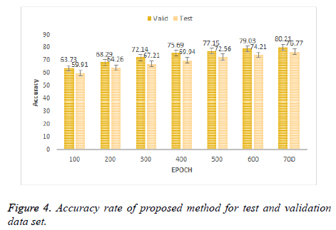
In Figure 4 the results of proposed method at different epochs. It can be seen that the classification results for three class classification obtained by proposed scheme is more pleasing as compared to the existing schemes in Figure 3. Proposed method achieved the accuracy of 80.21% and 76.77% on validation data set and test dataset respectively. Proposed method has improved the accuracy up to 19.23% on test dataset.
Conclusion
Mammograms classification for breast cancer detection based on CT and MLP is proposed. We have proposed a modal for the classification of breast tumour. We have found that MLP with DSIFT features can be used for the breast cancer detection. Numerical results shows that DSIFT features from the data set before inputting the data to the MLP is more helpful for cancer detection. Numerical results show the significance of our proposed method for large dataset of mammogram images as compare to other sate of art techniques. In future work, proposed method can be used with the combination of deep learning algorithms for high accuracy rate. Improvement can also be made by using different architectures of deep learning.
Acknowledgment
We have used the data set of IRMA group, Aachen, Germany, for this experimental study.
References
- Lee CH. Screening mammography: proven benefit, continued controversy. Radiologic Clin North Am 2002; 40: 395-407.
- American Cancer Society. http://www.cancer.org/cancer/ breastcancer/detailedguide/breast-cancer-detection, 2015.
- Abirami C, Harikumar R, Sannasi Chakravarthy SR. Performance analysis and detection of micro calcification in digital mammograms using wavelet features. Wireless Commun Sign Proc Network Int Conf IEEE 2016.
- Jasmine JL, Govardhan A, Baskaran S. Microcalcification detection in digital mammograms based on wavelet analysis and neural networks, in control, automation, communication and energy conservation, 2009. IEE Int Conf Energy Cons 2009; 1-6.
- Li Y, Houjin C, Xueye W, Yahui P, Lin C. Mass classification in mammograms based on two-concentric masks and discriminating texton. Patt Recogn 2016; 648-656.
- Mazurowski MA, Lo JY, Harrawood BP, Tourassi GD. Mutual information-based template matching scheme for detection of breast masses: From mammography to digital breast tomosynthesis. J Biomed Inform 2011; 44: 815-882.
- Casti P, Mencattini A, Salmeri M, Ancona A, Mangeri F, Pepe ML, Rangayyan RM.Contour-independent detection and classification of mammographic lesions. Biomed Sign Proc Control 2016; 165-177.
- Elter M, Hablmeyer E. A knowledge-based approach to the cadx of mammographic masses, in Medical imaging. Int Soc Optics Photonics 2008; 69150.
- Tao Y, Lo SCB, Hadjiski L, Chan HP, Freedman MT. Birads guided mammographic mass retrieval. SPIE Med Imag 2011; 79632.
- Muhammad TN. Classification of mammograms for breast cancer detection using fusion of discrete cosine transform and discrete wavelet transform features. Biomed Res 2016; 27: 322-327.
- Lin WC, Li CC, Christudass CS, Epstein JI, Veltri RW. Curvelet-based classification of prostate cancer histological images of critical gleason scores, in Biomedical Imaging (ISBI). IEEE 12th Int Symp 2015; 1020-1023.
- Eltoukhy MM, Faye I, Samir BB. Breast cancer diagnosis in digital mammogram using multiscale curvelet transform. Comp Med Imag Graphics 2010; 34: 269-276.
- Ucar A, Demir Y, Guzelis C. New facial expression recognition based on curvelet transform and online sequential extreme learning machine initialized with spherical clustering. Neur Comp Appl 2016; 27: 131-142.
- Bala BK, Audithan S. Wavelet and curvelet analysis for the classification of microcalcifiaction using mammogram images. Curr Trends Eng Technol Int Conf 2014; 517-521.
- Pinkus A. Approximation theory of the mlp model in neural networks. Acta Numerica 1999; 8: 143-195.
- Gonzalez RC, Woods RE, Eddins SL. Digital image processing using Matlab. Gatesmark Publ 2004.
- Candes EJ, Donoho DL. Curvelets, multiresolution representation, and scaling laws. Int Symp Optical Sci Technol 2000; 1-12.
- Ramachandran K, Soman K. Insight into wavelets: From theory to practice 2004.
- Eltoukhy MM, Faye I, Samir BB. A comparison of wavelet and curvelet for breast cancer diagnosis in digital mammogram. Comp Biol Med 2010; 40: 384-391.
- Candes E, Demanet L, Donoho D, Ying L. Fast discrete curvelet transforms, Multiscale Model Simul 2006; 5: 861-899.
- Lowe DG. Distinctive image features from scale-invariant keypoints. Int J Comp Vis 2004; 60: 91-110.
- Oliveira JE, Gueld MO, Araujo ADA, Ott B, Deserno TM. Toward a standard reference database for computer-aided mammography. Med Imag Int Soc Optics Photonics 2008; 69151.


