ISSN: 0970-938X (Print) | 0976-1683 (Electronic)
Biomedical Research
An International Journal of Medical Sciences
Research Article - Biomedical Research (2017) Volume 28, Issue 2
Comparison of different classification methods for the preictal stage detection in EEG signals
1Department of Electrical and Electronics Engineering, Sakarya University, Esentepe Kampusu, Serdivan Sakarya, Turkey
2Department of Electrical and Electronics Engineering, Institute of Natural Sciences, Sakarya University Esentepe Kampusu, Serdivan Sakarya, Turkey
3Department of Electrical and Electronics Engineering, Amasya University, Amasya, Turkey
- *Corresponding Author:
- Yildiz M
Department of Electrical and Electronics Engineering
Sakarya University, Turkey
Accepted on July 2, 2016
In this study, we present an evaluation and comparison of the widely used linear discriminant analysis, k-Nearest neighbor algorithm, support vector machines, multi-layer perceptron neural network and decision tree classification performances for preictal stage detection in EEG signal. Analysis has been done for fourteen patients with epilepsy. Firstly, 26 features are extracted from time domain, frequency domain and power spectrum. The feature set dimensionality has been reduced from 26 to 8 using Principal Component Analysis. Finally, five classifiers have been employed to classify EEG signals into normal, ictal and preictal stages. The classification is performed for patient-specific. We emphasized the importance of the analysis of preictal stage for seizure prediction. According to classification results and ROC analysis, Linear Discriminant Analysis and Support Vector Machines have better performances than others. LDA achieved the highest average sensitivity with 88.06% in the preictal stage detection process. The results are very promising and contributing to possible guide for future seizure detection and prediction studies.
Keywords
Epilepsy, Seizure detection, Seizure prediction, Classification method.
Introduction
Epilepsy is a common term including different types. It is characterized by seizures which occur at different and unforeseeable times without any symptoms. It causes discomfort in the central nervous system. Seizures are the temporary anomalies, cause abnormal electrical behaviour of a group of brain cells and can be detected by clinical signs and symptoms [1].
Electroencephalogram (EEG) signals are used commonly in epilepsy studies and diagnosis. EEG shows the representation of electrical activities generated by cerebral cortex neurons. For this reason, it is an important component in the clinic evaluation of brain activities, diagnosis of epilepsy and perception of epileptic attack. The EEG signals are acquired by placing necessary electrode to different centers and direct measures [1,2].
Starting to use the high-performance signal processing has caused to raise interests in such subjects as the phase of seizure, seizure detection and prediction. By using the many features extracted from EEG signals, it is aimed to separate the preictal phase, ictal phase, postictal phase and normal phase from each other. A great number of classifiers are used for this process [3].
Subasi et al. applied coefficients of autoregressive and Fourier into wavelet neuron network classifier and back propagation neural network classifier as input. They achieved 92.1% and 91.7% accuracy with seizure detection [4]. Srinivasan et al. proposed a seizure detection algorithm using recurrent neural network with time and frequency domain features [5]. Tzallas et al. analysed EEG sections using time-frequency distribution and then specified the features which represented energy distribution on time-frequency domain for each section. These features were classified using artificial neural networks [6].
Mirowski et al. performed SVM, Logistic Regression and Convolutional Networks for seizure prediction. They calculated bivariate features from pairs of EEG channels. They compared classification results. The results demonstrated that at least one method predicted 100% of seizures for each patient [7].
Hamid Vavadi et al. separated EEG signals as alpha, beta, theta, gamma and delta sub-bands by using wavelet transform. They calculated approximate entropies for EEG and sub-bands and classified these features using T-test [8].
Netoff et al. proposed the patient-specific algorithm for seizure prediction. This algorithm extracted spectral power in 9 bands from each of 6 electrodes. They achieved sensitivity of 77.8% (35 of 45 seizures) using Cost-Sensitive Support Vector Machines [9].
Abibullaev et al. used wavelet transform and wavelet threshold for feature extraction. Back propagation neural network had been implemented in order to classify and reached 94.69% accuracy with classify performance [10]. Shengi-Fu Liang et al. implemented seizure detection using approximate entropy, power and auto regressive model as feature. They applied genetic algorithms and principal component analysis to reduce feature. In the study, Linear Discriminant Analysis (LDA), back propagation artificial neural networks, linear least square and support vector machine (SVM) were used to classify EEG samples obtained different epileptic stage. Finally, they evaluated the results of classification for reduced feature set and all features, and compared the results with prior studies [11].
Subasi and Gursoy classified features based on discrete wavelet transforms. By using principal component analysis (PCA), independent component analysis and linear discriminant analysis, they reduced dimension of feature set. They achieved seizure detection without error with SVM classifier and linear discriminant analysis. [12].
Shoeb and Guttag suggested a method based on machine learning for seizure detection. They used SVM as classifier and compared system performances for patient-specific and patient-free [13]. Park et al. proposed the patient-specific algorithm for seizure prediction. Four different linear feature sets were generated from raw, time-differentiel, bipolar and bipolar/time-differential EEG signals separately. Their algorithm reached the best sensitivity of 97.50% with spectral power feature from bipolar EEG signals using Cost-Sensitive SVM [14].
Ozdemir and Yildirim developed an automated system epileptic seizure prediction based on Hilbert Huang Transform and Bayesian Classifiers. Their system successfully predicted seizure with sensitivity 96.55% [15].
Bandarabadi et al. proposed a system to reduce the number of false alarm for seizure prediction. They used relative combination of sub-band spectral powers as features to trace pre-seizure activities. They implemented feature selection based on amplitude distribution, and classified by SVM. They achieved sensitivity 75.8% [16].
The analysis of EEG signals is one of the most important and significant process in detection of epileptic stages. There have been great deals of methods to detect seizure in recent years. But most of previous studies didn’t focus on preictal stages. In this study, it has been investigated and evaluated the performances of five classifiers to detect not only normal and ictal stages but also preictal stages. In this study, a patientspecific algorithm which consists of feature extraction, dimension reduction and classification has been presented. The classification performances of Multi-Layer Perceptron Neural Network (MLPNN), Linear Discriminant Analysis, Support Vector Machines, k Nearest Neighbor (k-NN) and Decision Tree (DT) methods have been compared. We detected preictal stages with high accuracy for patient-specific cases. We intend to compare our results to previous studies in the literature. This study is very promising and contributing to seizure prediction studies. To the best of our knowledge, this study aims to propose seizure prediction method with high performance for further research.
Materials and Methods
EEG signals were taken from PhysioNet database [17]. The database contains scalp EEG signals of 24 patients. The international 10-20 system of EEG electrode positions and nomenclature was used for these recording. Database contains 198 seizures. The signals were sampled in 256 Hz with 16-bit resolution. Data contains stages of normal, preictal and ictal. The beginning time of seizures and total seizure durations in registration were remarked by the specialists.
In this paper, fourteen epilepsy patients are chosen considering the numbers of seizure and their durations. The preictal, ictal and normal stages were divided into 5 second periods. The preictal data has been taken from 80 second time intervals before the seizure's beginning time. The demographic information about the patients whose EEG signals consist the scope of this research is given in Table 1.
| Patient | Gender | Age | Patient | Gender | Age |
|---|---|---|---|---|---|
| Patient 1 | Female | 11 | Patient 8 | Female | 2 |
| Patient 2 | Female | 14 | Patient 9 | Female | 3 |
| Patient 3 | Male | 22 | Patient 10 | Male | 16 |
| Patient 4 | Female | 7 | Patient 11 | Female | 18 |
| Patient 5 | Male | 3.5 | Patient 12 | Female | 6 |
| Patient 6 | Female | 10 | Patient 13 | Female | 6 |
| Patient 7 | Male | 3 | Patient 14 | Undefined | |
Table 1. The demographic information of patients.
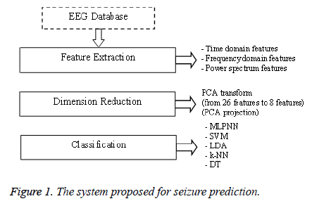
In this study, it has been proposed a system which contains three steps as feature extraction, dimension reduction and classification. Block diagram of the designed system is given Figure 1.
In the first step; twenty six features, widely used in the literature, are extracted from EEG signals. In the second step; principal components analysis has been performed for dimension reduction. In the third step; LDA, k-NN, SVM, MLPNN and DT have been employed for the classification.
The classification has been performed only patient-specific. Each step has been discussed with its sub-section in detail.
Feature extraction and dimension reduction
In this step of the study, a number of common features proposed in the literature have been selected. Feature set has been generated by calculating 26 features belong to time domain, frequency domain and power spectrum from EEG signals. These features are mean, mode, standard deviation, variance, minimum, maximum, zero cross rate, hjorth parameters (mobility, activity and complexity), renyi entropy, entropy, autoregressive coefficients (Burg-8 ones), total power, sub-band's power (alpha 1-2, beta, theta, gamma). The feature set dimensionality has been reduced from 26 to 8 applying PCA to decrease computational complexity. Then feature set has been divided into two parts as training set and testing set via cross validation method.
Classification
A great number of classification methods are used to detect stages of normal, ictal and preictal. In this study, LDA, k-NN, SVM, MLPNN and DT are used to classify.
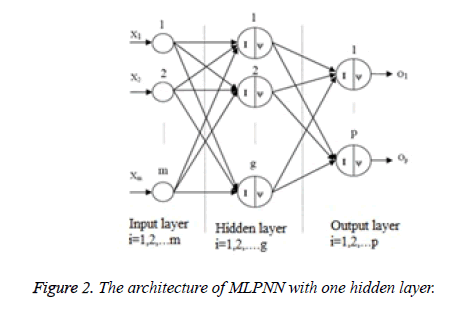
Multi-Layer Perceptron Neural Network (MLPNN): Multilayer perceptron includes an input layer, least one hidden layers and an output layer. Each layer has at least one neuron. MLPNN performs nonlinear mapping between input space and output space. MLPNN passes weights assigned to different layers, and determines the output and compares it with the desired output. Then it propagates error signal and adjust the connection weights correspondingly [18-20]. The architecture of MLPNN with one hidden layer is shown in Figure 2.
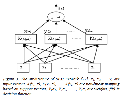
Support Vector Machines (SVM): SVM is a method for pattern classification which relies on the statistical learning theory. The formulation of SVM learning is based on the principle of structural risk minimization. SVM is based on the concept of decision planes that define decision boundaries. A decision plane is one plane that separates among a set of features having different class membership. SVM classifier finds the hyper-plane which maximizes the separating margin between classes. SVM defines class label of unknown data via function of classification (hyper-plane) by dividing data space. For this purpose, SVM uses most suitable separator hyperplane to divide the data [21-25]. Nonlinear SVM classifier is shown in Figure 3.
Figure 3: The architecture of SVM network [22]. x1, x2,....., xl are input vectors, K(x1, x), K(xx, x), ....., K(xn, x) are non-linear mapping based on support vectors, Y1α1, Y2α2, ……, Ynαn are weights, f(x) is decision function.
Linear Discriminant Analysis (LDA): LDA is one of the classification methods which are used in the fields of statistics and machine learning widely. LDA tries to provide more class separability and draws a decision region between the given classes. LDA searches for project axes on which the data points of the different classes are far from each other and the data points to the same class to be close to each other. LDA creates a linear combination of data sets which yield the largest mean differences between the desired classes [26-29].
K-Nearest Neighbour Algorithm (k-NN): k-NN is widely used classifier, instance-based on learning. This method is implemented by considering similarity of testing and training data. In the classification process, a sample is classified by a majority vote of its neighbors. Training data is represented in feature space. Each sample is a point in feature space. In this way, all of the training samples are stored in a feature space. When given an unknown sample, a k-nearest-neighbor classifier searches the feature space for the k training samples that are closest to the unknown sample. These k training samples are the k “nearest neighbors” of the unknown samples. For k-nearest-neighbor classification, the unknown sample is assigned the most common class among its k nearest neighbors [30,31].
Decision Trees (DT): Decision tree is a non-parametric supervised learning method. This method is widely used as classifier in many applications. It provides a model like tree structure which can be used to predict the class label of a target variable by learning simple decision rules inferred from classlabelled training data.
The classification process of testing samples is performed by sorting them based on feature values. Each node in a decision tree denotes a feature and each branch are generated by comparing testing value to a threshold value of the node. The topmost node is called the root node. All nodes excepted root node have exactly one incoming edge. A node with outgoing edges is called as internal node.
In a decision tree, each internal node partitions the feature space into two or more sub-spaces according to a certain discrete function of the input feature values. Classification is performed by tracing a path from the root node to a leaf node which has no outgoing edge. Each leaf holds a class label [31-33].
Results and Discussion
In the current study, we have tested a kind of patient-specific system for 14 patients in physionet database. 26 features are extracted for each patient from 21 channels.
Feature set dimensionality is reduced from 26 features to 8 features using PCA. Then the best channel has been determined via LDA classifier. In the rest of paper, we have used feature set belonging to the best channel for each patient. Training set and testing set are chosen from feature set via cross validation method.
The sample numbers of training and testing set and selected channels are given in Table 2.
| Sample Numbers | ||||||
|---|---|---|---|---|---|---|
| Stage | Normal Stage | Preictal Stage | Ictal Stage | |||
| Patient-Channel | training | testing | training | testing | training | testing |
| P1 P3-O1 | 128 | 64 | 75 | 37 | 58 | 30 |
| P2 P3-O1 | 128 | 64 | 74 | 38 | 52 | 26 |
| P3 FP2-F8 | 128 | 64 | 43 | 21 | 50 | 25 |
| P4 C3-P3 | 128 | 64 | 54 | 26 | 72 | 36 |
| P5 C4-P4 | 128 | 64 | 53 | 27 | 121 | 61 |
| P6 FT10-T8 | 128 | 64 | 43 | 21 | 37 | 18 |
| P7 C3-P3 | 128 | 64 | 75 | 37 | 58 | 30 |
| P8 T8-P8 | 128 | 64 | 118 | 58 | 74 | 36 |
| P9 FP2-F8 | 128 | 64 | 107 | 53 | 57 | 29 |
| P10 T7-P7 | 360 | 180 | 213 | 107 | 264 | 131 |
| P11 CZ-PZ | 128 | 64 | 64 | 32 | 42 | 22 |
| P12 C4-P4 | 128 | 64 | 85 | 43 | 40 | 20 |
| P13 F3-C3 | 128 | 64 | 75 | 37 | 56 | 28 |
| P14 FZ-CZ | 128 | 64 | 128 | 64 | 67 | 33 |
Table 2. Sample numbers and channels for each patient. Sample
LDA, k-NN, SVM, DT and MLPNN are applied to classify EEG signals into normal, ictal and preictal. Confusion matrices are constructed for the classifier performance evaluation. Then, accuracy, sensitivity and specificity are computed. These parameters are given in Table 3.
| LDA | k-NN | SVM | MLPNN | |||||||||
|---|---|---|---|---|---|---|---|---|---|---|---|---|
| pat | Sta | Sens. | Spec. | Acc. | Sens. | Spec. | Acc. | Sens. | Spec. | Acc. | Sens. | |
| P1 | Ict. | 100 | 100 | 100 | 100 | 100 | 100 | 100 | 100 | 100 | 100 | |
| Pre. | 100 | 100 | 100 | 100 | 100 | 100 | 100 | |||||
| Nor. | 100 | 100 | 100 | 100 | 100 | 100 | 100 | |||||
| P2 | Ict. | 100 | 98.04 | 97.66 | 100 | 98.04 | 96.09 | 96.15 | 99.02 | 97.66 | 100 | |
| Pre. | 92.11 | 100 | 86.84 | 100 | 94.74 | 98.89 | 84.21 | |||||
| Nor. | 100 | 98.44 | 100 | 95.31 | 100 | 98.44 | 100 | |||||
| P3 | Ict. | 76 | 94.12 | 80 | 68 | 98.82 | 85.45 | 72 | 98.82 | 82.73 | 68 | |
| Pre. | 85.71 | 83.15 | 71.43 | 98.88 | 80.95 | 91.01 | 66.67 | |||||
| Nor. | 79.69 | 95.65 | 96.88 | 69.57 | 87.5 | 78.26 | 90.63 | |||||
| P4 | Ict. | 91.67 | 98.89 | 92.86 | 88.89 | 98.89 | 89.68 | 88.89 | 97.78 | 90.48 | 91.67 | |
| Pre. | 88.46 | 97 | 69.23 | 97 | 76.92 | 95 | 80.77 | |||||
| Nor. | 95.31 | 91.94 | 98.44 | 85.48 | 96.88 | 91.94 | 87.5 | |||||
| P5 | Ict. | 91.8 | 96.7 | 94.74 | 96.72 | 98.9 | 93.42 | 98.36 | 98.9 | 95.39 | 96.72 | |
| Pre. | 92.59 | 100 | 70.37 | 100 | 77.78 | 100 | 62.96 | |||||
| Nor. | 98.44 | 94.32 | 100 | 89.77 | 100 | 93.18 | 98.44 | |||||
| P6 | Ict. | 94.44 | 100 | 95.15 | 94.44 | 100 | 91.26 | 94.44 | 100 | 96.12 | 100 | |
| Pre. | 90.48 | 97.56 | 76.19 | 95.12 | 85.71 | 100 | 80.95 | |||||
| Nor. | 96.88 | 92.31 | 95.31 | 87.18 | 100 | 89.74 | 98.44 | |||||
| P7 | Ict. | 93.33 | 100 | 87.02 | 96.67 | 99.01 | 83.97 | 96.67 | 100 | 89.31 | 96.67 | |
| Pre. | 75.68 | 93.62 | 62.16 | 93.62 | 72.97 | 96.81 | 37.84 | |||||
| Nor. | 90.63 | 83.58 | 90.63 | 79.1 | 95.31 | 83.58 | 92.19 | |||||
| P8 | Ict. | 91.67 | 99.18 | 96.2 | 75 | 99.18 | 92.41 | 88.89 | 100 | 96.84 | 94.44 | |
| Pre. | 96.55 | 98 | 94.83 | 96 | 98.28 | 96 | 81.03 | |||||
| Nor. | 98.44 | 96.81 | 100 | 92.55 | 100 | 98.94 | 96.88 | |||||
| P9 | Ict. | 89.66 | 98.29 | 85.62 | 79.31 | 97.44 | 80.14 | 82.76 | 98.29 | 83.56 | 89.66 | |
| Pre. | 77.36 | 93.55 | 75.47 | 90.32 | 69.81 | 96.77 | 56.6 | |||||
| Nor. | 90.63 | 84.15 | 84.38 | 79.27 | 95.31 | 76.83 | 90.63 | |||||
| P10 | Ict. | 90.08 | 97.56 | 87.8 | 89.31 | 98.26 | 89.47 | 92.37 | 96.86 | 90.19 | 92.37 | |
| Pre. | 74.77 | 93.89 | 75.7 | 95.18 | 72.9 | 96.78 | 69.16 | |||||
| Nor. | 93.89 | 89.5 | 97.78 | 89.92 | 98.89 | 90.76 | 92.78 | |||||
| Ict. | 90.91 | 100 | 89.83 | 90.91 | 100 | 84.75 | 90.91 | 98.96 | 85.59 | 86.36 | 90.63 | |
| Pre. | 75 | 96.51 | 56.25 | 96.51 | 59.38 | 96.51 | 40.63 | 95.35 | ||||
| Nor. | 96.88 | 83.33 | 96.88 | 72.22 | 96.88 | 75.93 | 93.75 | 75.93 | ||||
| P12 | Ict. | 95 | 100 | 99.21 | 100 | 100 | 100 | 100 | 100 | 100 | 95 | 100 |
| Pre. | 100 | 100 | 100 | 100 | 100 | 100 | 100 | 100 | ||||
| Nor. | 100 | 98.41 | 100 | 100 | 100 | 100 | 100 | 98.41 | ||||
| P13 | Ict. | 100 | 98.02 | 91.47 | 100 | 98.02 | 90.7 | 89.29 | 98.02 | 86.82 | 96.43 | 91.09 |
| Pre. | 91.89 | 91.3 | 83.78 | 93.48 | 72.97 | 94.57 | 54.05 | 96.74 | ||||
| Nor. | 87.5 | 98.46 | 90.63 | 93.85 | 93.75 | 84.62 | 90.63 | 81.54 | ||||
| P14 | Ict. | 75.76 | 99.22 | 85.71 | 75.76 | 99.22 | 79.5 | 75.76 | 100 | 85.09 | 84.85 | 88.28 |
| Pre. | 92.19 | 84.54 | 89.06 | 75.26 | 89.06 | 85.57 | 67.19 | 84.54 | ||||
| Nor. | 84.38 | 92.78 | 71.88 | 91.75 | 85.94 | 89.69 | 70.31 | 84.54 | ||||
Table 3. Classification performances.
It is observed that normal and preictal stages are interfered for each classifier. According to classification accuracies in the Table 3, SVM and LDA are more successful than k-NN, MLPNN and DT. Mean sensitivity values of all classifiers for preictal stage detection are given in Table 4. Table 4 demonstrated that LDA has produced the highest sensitivity over all classifiers.
| Classifier | LDA | k-NN | SVM | MLPNN | DT |
|---|---|---|---|---|---|
| Meansensitivity | 88.06 | 79.38 | 82.25 | 70.15 | 71.71 |
Table 4. Summary of results from five different classifiers.
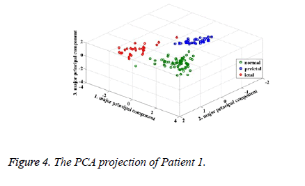
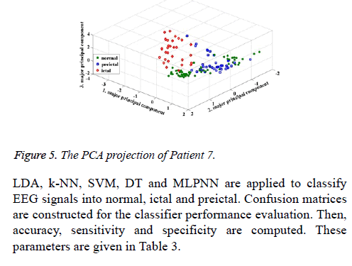
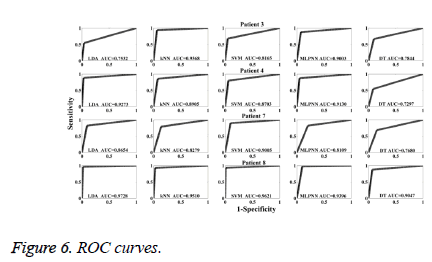
According to the PCA projections (Figures 4 and 5), it is observed that the normal, preictal and ictal stages are clearly separated from each other for Patient 1. At the same time, the preictal and normal stages are interfered in the projections for Patient 7. During the PCA projection, moreover, the clustering level of preictal stages is found as the best for Patient 1. The PCA projections approve classification results. For Patient 1, all classifiers achieved with 100% accuracy. In the classification result for Patient 7, from 9 to 19 preictal samples are detected as normal. In this study, ROC analysis is carried out to evaluate preictal stage detection performances of classifiers. ROC curves are shown for Patient 3, Patient 4, Patient 7 and Patient 8 in Figure 6. The values of Area under Curve (AUC) for all patients are given in Table 5.
| Patient | LDA | k-NN | SVM | MLPNN | DT |
|---|---|---|---|---|---|
| P1 | 1 | 1 | 1 | 1 | 1 |
| P2 | 0.9839 | 0.9737 | 0.9755 | 0.9688 | 0.9565 |
| P3 | 0.7532 | 0.9368 | 0.8165 | 0.9003 | 0.7844 |
| P4 | 0.9273 | 0.8905 | 0.8703 | 0.913 | 0.7297 |
| P5 | 0.9921 | 0.9699 | 0.9771 | 0.9349 | 0.8797 |
| P6 | 0.9402 | 0.8699 | 0.9824 | 0.9767 | 0.915 |
| P7 | 0.8654 | 0.8279 | 0.9005 | 0.8109 | 0.768 |
| P8 | 0.9728 | 0.951 | 0.9621 | 0.9396 | 0.9047 |
| P9 | 0.8756 | 0.8412 | 0.887 | 0.8528 | 0.7635 |
| P10 | 0.8617 | 0.8815 | 0.8992 | 0.8705 | 0.8105 |
| P11 | 0.9005 | 0.8564 | 0.8641 | 0.7883 | 0.7847 |
| P12 | 1 | 1 | 1 | 1 | 0.9824 |
| P13 | 0.8875 | 0.8863 | 0.8703 | 0.8546 | 0.8122 |
| P14 | 0.8699 | 0.8081 | 0.8625 | 0.7687 | 0.7481 |
| mean | 0.9164 | 0.9067 | 0.9191 | 0.8985 | 0.8457 |
Table 5. The values of area under curve (AUC) for preictal stage detection.
ROC curves and AUC values show that LDA outperformed the other four classifiers for most of patients during the preictal stage detection. For comparison SVM has better performances than k-NN, MLPNN and DT. DT is the worst classifier in the preictal stage detection process. According average AUC values, SVM has the best performance.
Conclusion
Throughout the review of literature, it has been observed that many studies have been performed to detect epileptic seizure from EEG signals. In these studies, researchers proposed different methods with high performance. Moreover, error-free methods were developed capable of separating ictal and normal periods from each other. The evaluation of the preictal periods is inevitable in order to avoid the patients from the possible seizure and its possible caused negativities and improve the life quality of them. Therefore, preictal stage has an important role for seizure prediction.
Thus, the objective of this paper is to evaluate not only the normal and ictal stages as the previous studies focused on but also the preictal stages which have been taken into consideration during the analysis of EEG signals. Since the characteristics of epilepsy differs patient specifically, EEG signals have been analysed for patient-specific.
In this paper, a system is designed to compare five different classification methods for seizure prediction. We performed the classification of EEG signals into normal, ictal and preictal stages. Classification rates indicate that LDA and SVM outperform the other classifiers. It is found that LDA results are more successful than SVM to detect preictal stages. It is clearly observed that PCA projections confirm classification results. Both classification results and PCA projections show that it is more difficult to classify normal and preictal stages. In addition, ictal stages are well separated from other stages.
Several seizure prediction systems were designed in the literature. In [9,14-16] they used Freiburg Database which contains intracranial EEG (iEEG) recordings. They classified EEG signals into preictal and interictal stages using multichannel EEG signals. They obtained sensitivity of 77.8%, 97.5%, 96.55% and 75% respectively. In these studies, researchers used one classification method. In [7], researchers compared logistic regression, convolutional networks and support vector machine performances to classify EEG signals into preictal and interictal. They obtained that for each patient at least one method predicted 100% of seizure on Freiburg dataset.
On the other hand, this study and previous studies are not easily comparable, because EEG data sets are different. They classified EEG signals as preictal and interictal. We classify EEG signals as normal, preictal and ictal. On the contrary to the previous studies [9,14-16] which used one classifier, this paper is a comprehensive and comparative study that aims to detect preictal stage using LDA, k-NN, DT, MLPNN and SVM classifiers.
We used different EEG database which contains scalp EEG in contrast to intracranial EEG recordings used in the previous studies. For five classifiers, results are compared and it is found out that LDA and SVM have the best results among the abovementioned classifiers. LDA achieves the highest average sensitivity with 88.06% to detect preictal stage.
Results indicate that normal and preictal stages are interfered. Therefore, researchers had better consider the description of the discriminative features for normal and preictal stages. In this study, mainly the separation of preictal stages from others has been analysed. PCA projections, ROC curves and AUC values, which signify the system performance, confirm the results of the classification. With these results, it is hoped that the application of seizure prediction technologies will be more successful in future and shed light on further studies.
Acknowledgement
This research was supported by Sakarya University Scientific Research Projects Commission (Project Number: 2013-50-02-010).
References
- Sivasankari N, Thanushkodi K. Automated epileptic seizure detection in EEG signals using FastICA and neural network. Int. J. Advance Soft ComputAppl 2009; 1: 1-14.
- Subasi A. Epileptic seizure detection using dynamic wavelet network. Exp sys appl 2005; 29: 343-355.
- Ouyang G, Li X, Li Y, Guan X. Application of wavelet-based similarity analysis to epileptic seizures prediction. Comp Biol Med 2007; 37: 430-437.
- Subasi A, Kalkan A, Koklukaya E. EEG isaretlerinindalgac?ksiniragiiles?niflandirilmasi. Teknoloji 2004; 7: 71-80.
- Srinivasan V, Esweran C, Sriraam N. Artificial neural network based epileptic detection using time-domain and frequency-domain features. JMed Sys 2005; 29: 647-660.
- Tzalles A Z, Tsipouras M G, Fotiadis D I. Automatic seizure detection based on time-frequency Analysis and artificial neural networks. Comput IntelNeurosci 2007; 2007: 1-13.
- Mirowski PW, LeCun Y, Madhavan D,Kuzniecky R. Comparing SVM and convolutional networks for epileptic seizure prediction from intracranial EEG. Iee Mach L Sig Proc 2008; 244-249.
- Vavadi H, Ayatollahi A, Mirzaei A. A wavelet-approximate entropy method for epileptic activity detection from EEG and its sub-bands. J. Biomed SciEng 2010; 3:1182-1189.
- Netoff T, Park Y,Parhi K. Seizure prediction using cost-sensitive support vector machine. 2009 Annual International ConfEng Med BiolSoc 2009; 3322-3325.
- Abibullaev B, Seo HD, Kim MS. Epileptic spike detection using continuous wavelet transforms and artificial neural networks. World SciPubl Comp 2010; 8: 33-48.
- Liang SF, Wang HC, Chang WL. Combination of EEG complexity and spectral analysis for epilepsy diagnosis and seizure detection. Eurasip J Adv Sig Proc 2010; 2010: 1-15.
- Subasi AH, Gursoy MI. EEG signal classification using PCA, ICA, LDA and support vector machines Exp Sys Appl 2010; 37: 8659-8666.
- Shoeb A, Guttag J. Application of machine learning to epileptic seizure detection. IntConf Mach Learn 2010; 975-982.
- Park Y, Luo L, Parhi KK, Netoff T. Seizure prediction with spectral power of EEG using cost-sensitive support vector machines. Epilepsia 2011; 52: 1761-1770.
- Ozdemir N, Yildirim E. Patient specific seizure prediction system using hilbert spectrum and bayesian networks classifiers.HindawiPubl Corp 2014; 2014:1-10.
- Bandarabadi M, Teixeira CA, Rasekhi J, Dourado A. Epileptic Seizure Prediction Using Relative Spectral Power features. ClinNeurophysiol 2015; 126: 237-248
- International database www.physionet.org.
- Meyer-Baese A. Pattern recognition for medical imaging. California Elsevier AcadPres 2004.
- Haykin S. Neural networks: A comprehensive foundation. New Jersey Pren H 1999.
- Zurada JM. Introduction to artificial neural systems. St Paul West Publ Comp 1992.
- Zheng N, Xue J. Statistical Learning and Pattern Analysis for Image and Video Processing. SprinVerl 2009.
- Vapnik VN. Statistical Learning Theory. New York W Intersci 1998.
- El-Naqa I, Yang Y, Wernick MN, Galatsanos NP, Nishikawa RM. A support vector machine approach for detection of microcalcifications. Ieee Trans Med Imag 2002; 21: 1552-1563.
- Abe S. Support vector machines for Pattern Classification. New York Sprin 2005.
- Burges CJC. A tutorial on support vector machines for pattern recognition. Data Mining and Knowledge Discovery. Boston Kluwer AcadPubl 1998.
- Junoh AK, Mansor MN. Safety system based on linear discriminant analysis. InstMeasSens Net Autom 2012; 32-34.
- Panahi N, Shayesteh MG, Mihandoost S, Zali-Varghahan B. Recognition of different datasets using PCA, LDA, and various classifiers.Appl InformCommTechnol 2011; 1-5.
- Unsal A. Diskriminantanaliziveuygulamas?uzerinebirornekGuiibfDergisi 2000; 2: 19-36.
- Fielding A. Cluster and Classification Techniques for the Biosciences. New York CambrUni2000.
- Mitchell TM. Machine learning. McGraw-Hill SciEngMath 1997.
- Han J, Kamber M. Data Mining Concepts and Techniques. Morgan Kaufmann (3rd edn.) 2012.
- Maimon O, Rokach L. Data Mining and Knowledge Discovery Handbook. Spr New York 2011.
- Kotsiantis SB. Supervised Machine Learning: A Review of Classification Techniques Informatica 2007; 31: 249-268.
