ISSN: 0970-938X (Print) | 0976-1683 (Electronic)
Biomedical Research
An International Journal of Medical Sciences
Research Article - Biomedical Research (2017) Artificial Intelligent Techniques for Bio Medical Signal Processing: Edition-I
Detecting and classifying ECG abnormalities using a multi model methods
1Department Electronics Engineering, Sathyabama University, Solinganallur, Tamil Nadu, India
2Deaprtment of Electronics Sciences, Bharath University, Chennai, Tamil Nadu, India
- *Corresponding Author:
- Mahalakshmi Ponnusamy
Department Electronics Engineering
Sathyabama University, India
Accepted on January 13, 2017
Heart Abnormalities can be diagnosed accurately by examining and investigating the ECG signals carefully. Numerous techniques were proposed in the earlier research works in the area of arrhythmia detection by utilizing traditional methods of classification. Also, in the earlier researches Chaos theory and non-linear analysis are applied to characterizing the ECG signals. In this paper, the proposed method detects and analyses the abnormalities with respect to P, Q, R and S peak values. The entire proposed work is divided into three phases, whereas in the first phase, the data acquisition is applied to the real time ECG data. In the second phase, preprocessing is applied to the ECG signal data. In the third phase, features are extracted from ECG signals and finally from the extracted features, the abnormal peaks are classified to identify the abnormality of the ECG signals. The data acquisition is achieved from the relevant database, then preprocesses the data using Base Line Correction (BLC), inflection point detection using Powerline interference, Feature Extraction by GLCM method and finally features are classified and detecting the abnormality using the SVM classifier. The data set used in this paper is taken from the world-famous MIT-BIH Arrhythmia database and other international ECG signal databases.
Keywords
Signal processing, Feature extraction, SVM classifier, Base line correction, ECG signal, Morphological operation.
Introduction
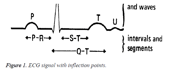
ECG-ElectroCardioGram is one of the famous diagnosing tools which measure the electrical activities of the heart and record the details. The recorded details are interpreted to diagnose the heart conditions [1,2]. It is well known that the current is diffused around the body surface. At the same time ECG is generated by the nerve impulse additional to the heart. A voltage drop is built by the current in the body, where it converts the microvolt into millivolt with an impulse variation. The number of amplification on the impulse should be more number of times. Generally an ECG shows normal heart rate consists of a P-Wave, QRS complex and a T-Wave depicted in Figure 1. 50% to 75% of the ECGs are represented in a small U wave. The baseline is called as isoelectric line. Typically, the isoelectric line is measured as the portion of tracing following the T wave and preceding the next P wave. The electrical activity of the heart can be recorded at the surface of the body using an Electrocardiogram. Therefore, the electro-cardio-gram (EKG) is simply a voltmeter that uses up to 12 different leads (electrodes) placed in designated areas of the body.
Most of the human diseases are analyzed by medical image processing techniques only. Human brain problems can be detected and classified by diagnosing MRI (Magnetic Resonance Imaging) images [3]. But diseases related to human heart are diagnosed by Electrocardiogram waves only. The electrocardiogram is a diagnostic tool that is used to study the human heart’s electrical activities with accurate measures. Based on these studies about heart’s electrical activities several heart diseases can be diagnosed. According to different studies [1,2] the diseases of any severity from the beginning stages of the disease to severe stages can be diagnosed by studying the ECG signals. Without any electrocardiography analyzers the efficiency of medical instruments in diagnosing the diseases using hearts activities would not be as better as they are with employing them [4]. The ECG analyzers extract the useful information from the signals generated from the heart’s electrical activity precisely. In another study MATLAB was used to test and filter noise in the ECG signals as the ECG signals are generally very noisy, to obtain better ventricular depolarization in the recorded signals [5]. As the ECG signals are generally very noisy, the signal must undergo processing in order to reduce the effects of noise. The ECG signal processing consists of two stages, namely preprocessing and feature extraction. In the preprocessing stage the noises in the raw ECG signal are suppressed or removed. The feature extraction process obtains diagnostic information contained in the preprocessed ECG signal. According to a study by Correia [6] the feature obtained from the preprocessed ECG is termed as a form. In preprocessing stage there are several noises are suppressed, according to a study by Carr and Brown [7] the contaminants can be specifically categorized as follows:
• Electromyography (EMG) noise
• Patient-electrode motion artifacts
• Power line interference
• Baseline wandering
• Electrode pop or contact noise
The fact that the biological signals comprise of other disturbances among them due to artifacts or physical interference from the surroundings made Clayton [8] to try techniques such as Fourier Transform (FT) for analysis of these signals using frequency domain techniques. In a study by Wood and Barry [9] it is stated that the ECG signals like other biological signals belong to the multicomponent non stationary kind of signals. So obtaining an accurate time varying spectral estimate will be a very difficult process. In different studies the Time-Frequency analysis is used to overcome this problem by using a uniform Time Frequency Distribution (TFD) [10,11]. In order to perform time-frequency analysis the concept of instantaneous frequency plays a vital role. The concept of Instantaneous Frequency is discussed thoroughly in various studies [12,13]. There are several conventional techniques used for analysis of ECG signals. In a study by Goy et al. [14], it is discussed that a systematic analysis of the surface ECG which is a critical task in ECG analysis. The author presented that the conduction of abnormalities modifies the T wave while depolarization is abnormal. The variation of QT interval shows the tachycardia. Bacharova et al. [15], utilized a traditional approach for diagnosing ECG. Through ECG criteria, it is easy to analyze the LVH and LVM. In study by Guillén et al. [16], autocorrelation function is used to detect arrhythmia whereas it refers the frequency domain features are used in another study [17]. The time-frequency analysis is taken from different studies [18-20] and apart from these conventional techniques some other techniques such as adaptive filtering and sequential hypothesis testing are also used for ECG analysis [21-23].
From the above background study, it is clear that the removal of noise in an ECG signal is very much important in bio-medical signal processing. Also the earlier research works of ECG signal processing were done with respect to time domain. Extracting the features from the ECG signal requires more than the time domain. ECG implementation is signal processing in terms of digits.
Normal ECG signal
Generally the frequency range of the ECG signal is from 0.05 Hz to 100 Hz with the duty range of 1 mV to 10 mV. The number of peaks and valleys in the ECG is represented by the alphabets as P, Q, R, S and T [24]. Sometimes one more peak is also used as U. ECG is analyzed with the help of detecting the accurate and reliable detection of QRS complex integrated with T and P waves. The activation of the upper chambers of the heart [atria] is represented by P-waves during the QRS complex. The excitation of the lower channel called as ventricles of the heart is represented by T-waves. Detecting and analyzing the QRS complex is the main task of analyzing the ECG signal. Once the QRS complex is identified, then the investigation of ECG signal is applied with the heart rate. The P-R, Q-T, and QRS intervals range of the normal state heart and abnormal state heart rate is given in the following Table 1.
| Amplitude | P-Wave | .25 mV |
| R-Wave | 1.60 mV | |
| Q-Wave | 25% of R wave | |
| T-Wave | .1 to .5 mV | |
| Duration | P-R interval | .12 to .20 sec |
| Q-R interval | .35 to .44 sec | |
| S-T interval | .05 to .015 sec | |
| P-Wave interval | .11 sec | |
| QRS interval | .09 sec |
Table 1. Values of the normal heart rate.
According to the values given in Table 1 and from the shape of the ECG recorded, it is easy to say that the heart activity is normal or abnormal.
Abnormal ECG signal
The abnormal value of the heart beat does not lie between the ranges of 60 to 100 beats/ minutes. Slower rate than 60 beats/min represents a lower heart rate and it is called as bradycardia. The higher rate of the heart beat than 100 beats/ min is a fast heart rate and it is called as tachycardia. If the cycle space is not even then it indicates an arrhythmia. Arrhythmia is indicated by verifying the cycles. Also, if the P-R interval is greater than 0.2 seconds, then it is suggested as blockage of the AV node. The heart valves are not diagnosed by ECG, it is diagnosed using other techniques like angiography and echocardiography which provide information not in the ECG. ECG is segmented horizontally and P-wave is obtained and nominated at the baseline. Now the QRS complex becomes the combination of depolarization of the atria and depolarization of the ventricles and both occur simultaneously. T-waves reflect the rhythmic electrical depolarization and repolarization of the myocardium associated with the contractions of the atria and ventricles. This ECG is used clinically in diagnosing various abnormalities and conditions associated with the heart. From this it is clear that the duration and the morphology of the QRS complex help to diagnose the cardiac arrhythmias, abnormalities of the heart and other disease states.
Materials and Methods
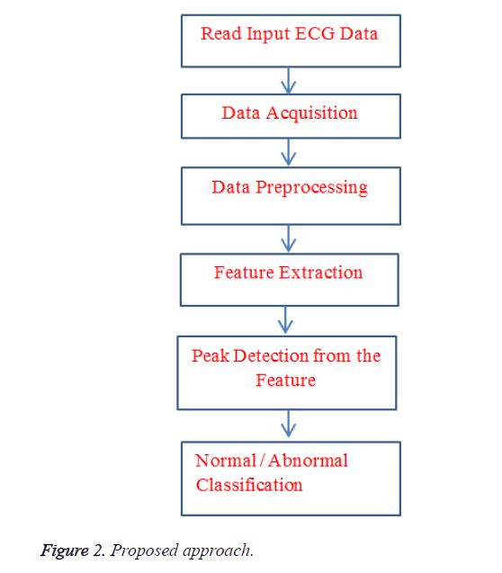
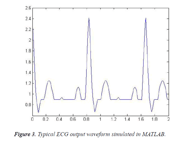
The main objective of the ECG simulator is to produce common ECG waveforms with different leads and with arrhythmias. Using the MATLAB software the simulator is able to produce the normal ECG waveform [25-28]. There are more advantages of using this simulator since it has more advantages in the simulation of the ECG waveforms The main advantages of our ECG simulator is to save the time and removing the hazards while recording the ECG using invasive and non-invasive methods (Figure 2). The common and features of the ECG signal are P, Q, R, S and T waves and the relevant intervals such as P-R, S-T and Q-T intervals. The periodic interval is determined by the heartbeat. Figure 1 shows the model of an ECG waveform, from this figure, it is clear that an ECG wave is a combination of a triangle and sinusoidal wave forms. In QRS, Q and S portions of the ECG is represented by triangular waveforms. In P, T and U portions are represented by triangular waveforms. After generating each portions all are integrated finally to obtain the ECG signal. A typical ECG waveform is shown in Figure 3.
The specifications of the ECG signal are default and it can also be changed due to the user’s requirement. The heartbeat is taken as 73 amplitude of P, Q, R, T waves as 25 mV, 1.6 mV, 0.025 mV and 0.35 mV with respective to the intervals P-R, S-T, P and QRS interval as 0.16 s, 0.18 s, 0.09 s, 0.11 s respectively. From the world famous MIT-BIH arrhythmia database there are two hundred ECGs are taken from experiment. This database consists of 109000 beats are annotated manually. All the signals are sampled at 360 Hz.
Data acquisition
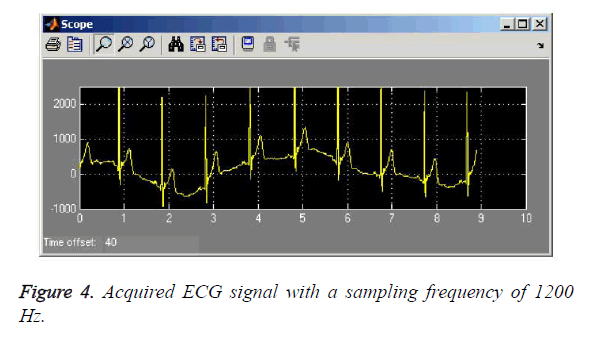
By utilizing the Data Acquisition Toolbox and blocks available in the toolbox the real time data is acquired into the Simulink model and the final signal is output into a physical hardware. Analog input blocks to acquire live data from a data acquisition device into Simulink. The acquired data is processed and produced as an ECG output. The output of the data acquisition is fed into Simulink blocks for analog data processing. The recorded ECG signal is having noise and artifacts often because of similar characteristics. In order to remove the noise from the ECG signal it is essential to process the raw data from the ECG signal (Figure 4). The main functionality of the ECG signal comprises of two stages such as preprocessing and feature extraction. The preprocessing of the signal removes or suppress the noise in the raw ECG data and feature extraction methods extracts the diagnostic information available in ECG signal.
Data preprocessing
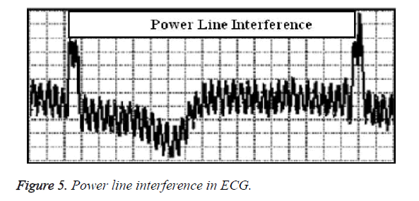
ECG consists of various kinds of noise such as Power line interference, Electrode pop or contact noise, Patient-electrode motion artifacts, Baseline wandering and Electromyography (EMG) noise. Within these noises the power line interference and the baseline wandering are the most common and affect the analysis of the ECG strongly. Other noises are wideband and complex in nature and distort the ECG signal. Powerline noise is centered at 60 Hz with a bandwidth of equal or lesser than 1 Hz and it will be removed during the acquisition process itself. Other noises are removed by efficient software methods. To do a baseline correction, it is necessary to acquire the perfect ECG signal without BW, ECG signal with knowing BW and a real ECG combined both. From the PhyisoNet website (www.physionet.org/pn3/twadb/) contains research oriented database includes T-wave alternans challenging database. All datasets are having 100 multichannel ECG records sampled at the frequency of 500 Hz with 16-bit resolution over an ± 32 MV range. All the information about the data is stored in the form of *.hea format. From the database twa18 and twa34 data are chosen for the experiments. Since these datasets (Channel-I) has perceptual isoelectric level baseline and any standard ECG can be replaced by a segment of an ECG signal from the twa34 (channel-I). The selected ECG signal consists 11 ECG cycles with last 6 s (Figure 5). ECG signal in twa18 channel-III has severed contaminated by BW.
Thus, the ECG signal available in twa18 channel-III is used as the real contaminated ECG signal to verify the performance of the proposed approach. Electrode-skin impedance gets changed due to patient’s movement and perspiration. Similar to the communication-modulation ECG amplitude is acquired through the electrode varies with the impedance changes. This type of BW is simulated using Gaussian model [27] and formulated as:
 (1)
(1)
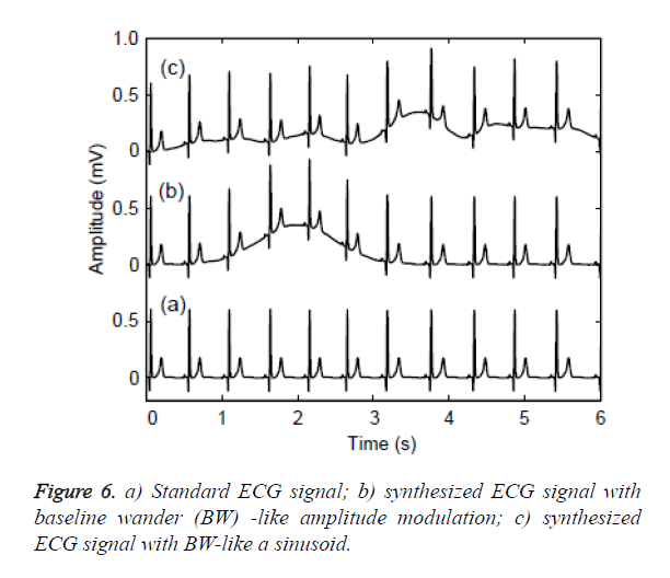
where bl(i) is the ith BL value, A is the peak value obtained the appropriate peak time p and s is the amplitude changing rate of BL. Figure 6b shows the synthesized ECG signal with BW-line amplitude modulated. In this paper the baseline interference is also corrected by using a polynomial curve fitting algorithm. The entire signal is fitted and then the original signal is subtracted from this polynomial to set the baseline correction to zero. The polynomial equation is:
 (2)
(2)
The first differentiation gets the first level of the peak or valley value in the ECG signal. Fixed equation cannot filter all the peak or valley values. To solve this problem a threshold value is assigned to grab the fall or raise values from the ECG signal.
By assigning a threshold value the R wave is extracted from the upper side and S wave from the opposite side. Using this other features can also be extracted. This process is obtained by rearranging the peak or valley values of the ECG in ascending order, where the threshold is the center between the highest differences between them. Peak value is obtained by detecting the change from positive to negative values in the wave. The valley is obtained by detecting the change from negative to positive values in the wave.
Power Line Interference
During ECG recording the most common are Powerline interference and baseline drift. It is easy to recognize the power line interference, if the interfering voltage in the ECG is less than or equal to 50 Hz of frequency. Interference occurs due to loops in the patient’s cable or wandering effects in the alternate current fields. It also happens due to a loose connection on the cable or due to dirty electrodes or due to not grounded properly. But the most general reason of 50 Hz interference is the disconnected electrode produce a strong disturbing signal and it need very fast action. The quality of the ECG is also affected by the electromagnetic interference, electric equipment in the room such as air conditioner, air cooler elevators and X-Ray units etc. These electrical devices draw heavy power, including 50 Hz signal in the input circuit of the ECG machine. It also happens due to switching acting in the electrical power systems. From the above to suppress the transients, it is essential to take care and the ECG with power line interference is shown in Figure 6.
To detect accurately it essential to filter out or eliminate all the noise sources. These problems can be dealt with analog filters. Analog filters introduce nonlinear phase shifts, skewing the signal. But digital filters are good and capable to implement and bring more advantages than analog filter and also digital filters are more precise because of less instrumentation. Nowadays digital filters are the most one used in recent research and medical fields. In this paper FIR Notch Filters are used to correct the power line interference. Linear-phase equiripple filters are desirable since they have very less maximum deviation from the ideal filter comparing with all other linear-phase FIR filters of the same order. This filter utilizes the windowing method to fetch the desired frequency response with the less number of coefficients. The selected frequency is compared with the actual frequency and obtains the solution where the comparison is done iteratively. This equiripple filter is deigned based on an optimization theory and it needs an enormous amount of computational effort. Since the convergence rate is high. The efficiency of the FIR filter is computed by de-noising measured by SNR of the enhanced signal. SNR can be computed by
 (3)
(3)
Where, xoriginal-xdenoised is the difference between the raw ECG and the filtered ECG signal.
Inflection point detection
P, Q, R, S, T and U have inflection point throughput and the whole signal is shown in Figure 1. Initially R, S waves are extracted to determine the R-R interval and estimate the heart rate. By correcting the baseline correction and building an automatic threshold the R wave is detected as the highest value in the ECG by differentiating the point values higher than the threshold value. The period between two consecutive R waves is detected as the R-R interval. Also the heart rate is counted from the beats within a stipulated period. The heart rate can be calculated as:
 (4)
(4)
Q and S wave detection
From the R-R interval S and Q waves are detected by dividing the R-R interval into four equal groups. Q values can be extracted as the valley directly before R wave. S waves are extracted as the biggest valley directly after R waves which is shown in Figure 4.
QRS complex detection
It is easy to determine the QRS complex from the known R, Q and S waves because the three values are the three following inflection points. QRS interval is the result from subtracting the S and Q waves.
T wave detection
It is clear and observed that the most distortion periods in the ECG is between Q and S waves. There are more inflection points should be filtered to get the necessary inflection points that referred to P and T-waves. To avoid taking wrong peak values, smoothing ECG has been applied; since smoothing stopped after 15 peaks or valley then it assumes that it is the highest peak or valley in the first half of the regions directly after S wave.
P wave detection
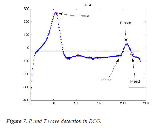
After smoothing still some more number of peaks and valleys reaches 6, and it is assumed as the highest peaks in the second half regions directly before Q wave and it is shown in Figure 7.
S-T detection
The points between the S and T waves are stored negatively and positively to their places from the baseline to define which of them has more points than the other and it is shown in Figure 7.
QT detection
QT interval is the result obtained by subtracting Q and T waves and it is shown in Figure 7.
PR interval
From beginning of the P wave in the beginning of the QRX complex is measured as PR interval and it is shown in Figure 7.
Feature Extraction using Gray Level Co- Occurrence Matrix
Gray Level Co-occurrence Matrix and Support Vector Machine are the machine learning approach is utilized for feature extraction and categorization. GLCM based features are extracted from the ECG signals and SVM is used for classifying the features. Feature extraction, reducing the amount of data which makes accuracy in classification and reduce the time. GLCM extracts the features such as Mean, Energy, Correlation, Skewness and Kurtosis and their formulas are given below.
 (5)
(5)
 (6)
(6)
 (7)
(7)
The GLCM algorithm is written below:
Steps for GLCM:
Step 1: Read the ECG data from the users
Step 2: Read the content of the ECG from .dat file
Step 3: Calculate the co-occurrence matrix
Step 4: Calculate Haralick texture features
Step 5: Save acquired information to a database file.
Classification using support vector machine
Classification refers the features and the properties of the ECG signal. All the features are analyzed and classified into two groups as 0 and 1 [True and false]. To do classification training and testing process on the ECG data is applied. Training phase takes the known data with the classified label and the test phase takes the unknown data to be tested and comparing with the trained data results. In this paper classification of ECG data is obtained by the SVM method described below.
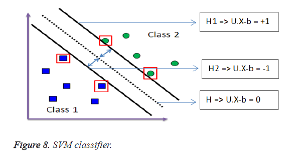
Support vector machine is used commonly on linear and non-linear data. SVM utilizes a non-linear mapping method to do the transformation. It transforms the training data into a higher dimension. All data are classified into two classes as 0 or 1. SVM searches the linear optimal boundary with new dimensions. It finds a hyperplane and defines a margin with the help of the support vectors. To train the data numerous classes are created by drawing a plane among the training points. SVM, KNN and perception are some of the methods used for classifying linear and non-linear data. Among various numbers of Hyperplanes, any one hyperplane be the decision boundary. To choose the optimum hyperplane, the margin of each hyperplane is verified. Hyperplane having the maximum margin is selected as the best hyperplane for classification. In Figure 8, the dotted lines are decision boundaries separating the parallel lines. The distance between the dotted lines is called as margin. The width of the margin is called as support vectors. Three hyper planes are considered which touches high, medium and low boundaries of the planes. Here linear state vector is obtained by the continuing distribution function.
The unknown data are “x” and the sum of similar support vectors is represented as (xi). The similarity value is the dot product of the “x” and “xi”. The following equation verifies the coefficient of the support vector (α) controls the contribution of a specific support vector. The result of a single support vector is defined by the following function as:
 (8)
(8)
Where l be the length of the support vectors and yi is the class of the corresponding support vector.
The very common SVM algorithm used for data classification is given below where as it is used in this paper to classify the ECG data.
Algorithm for SVM Classifier:
/**
*This algorithm solves the classifier problem by calling
*Set of points in the SV array.
*
*Input: Input data matrix from ECG data
*Output: Set of support Vectors segmented
*Initialization: Error threshold = huge value
**/
begin
Randomly sample 2 data belongs to different classes.
Add them to current set of SV
Set the corresponding variables (‘α’) values
Loop SVm
Loop to randomly consider other samples
Choose the set of points with which current SV gives sample
point Less than the Current error threshold.
End loop random sample some other ECG data
Update error threshold as average of sampled test errors.
Loop over misclassified points
Add the point to current SVs
Train the data set over the remaining ECG data.
End loop over misclassified points
Save variable (‘α’) for next iteration
End Loop SVm
End
Results and Discussion
The entire process of the proposed approach is implemented in MATLAB software and tested with MIT-BIH datasets. The entire data is preprocessed, feature extracted and classified as normal or abnormal ECG signal. Since the data set is tested and verified by most of the researchers and students in the world, it is easy to compare the obtained results with the real time as well as template based results. The performance can also be calculated by comparing the results of the proposed approach with the earlier research based results. The entire dataset is divided into two portions as train and test data. The classified label of the training data is known and the test data results are compared with that. There are various classification methods such as supervised and unsupervised learning approaches. Those methods utilize the labels for classification. All the signals are taken from the MIT-BIH arrhythmia database and all are annotated by cardiologists (experts) available in “signal.dat”. The obtained results shown in two-dimension only.
The experimental results obtained from MATLAB software are given here and discussed. We extracted totally 10 features and tested from ECG signals in 100 ECG samples which represent normal or abnormal waves. The features are P, Q, R, S, QRS, T, ST, PR, QT and PR. After extraction, it is performed 84 tests and had 89 significant and 11 insignificant in the data. We applied SVM classifier. The average of all the features (significant as well as insignificant) is given to the classifier initially. Then only the significant features are classified. Then only a sample data of a patient is given at a constant time interval. Finally, three samples from the same patient giving the entire ECG signals are classified.
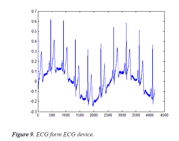
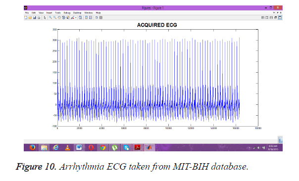
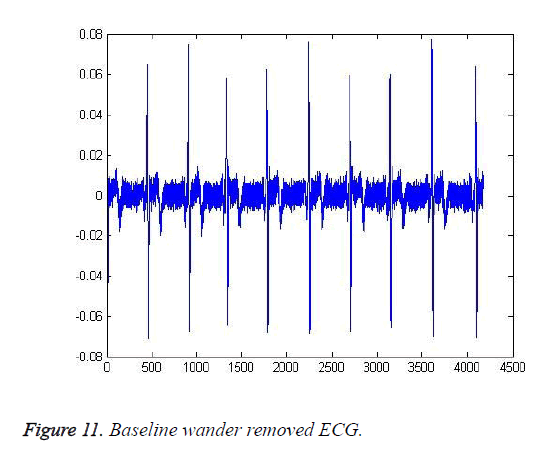
Figures 9 and 10 shows the normal ECG and arrhythmia ECG taken from another database and the MIT-BIH database respectively. According to our proposed approach architecture, noise removed, baseline correction and power line interference are processed one by one like signal processing application. Any ECG inputs taken from ECG devices or from software generating an ECG through data stored in a file can generate ECG waveforms look like Figure 9 only. The Baseline wanders is removed with the help of baseline correction methodology and the results are shown in Figure 11.
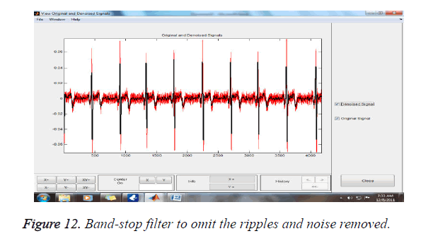
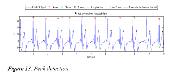
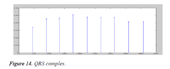
Figure 12 shows the ripples and noise removed signal. The band-stop method removes the noise and ripples and Figure 13 shows the peak values detected in an ECG and Figure 14 shows the QRS complex fetched in the signal with the help of feature extraction method. The amplitude of decreased signal is also improved in reference of the original signal. The result obtained in de-noised signal helps the experts diagnose the diseases more accurately. From the experiment the ECG signal is used clinically in diagnosing several abnormalities and constraints related with the heart. The statistical information in Table 1 is referred in this paper to justify the obtained output.
It is well known that the normal heart beat lies within the range of ≥ 60 to ≤ 100 beats per minute. A low rate than this range is called as Bradycardia, that is low heart and higher rate is called as tachycardia that is fast hear. An arrhythmia is indicated by non-even spaces whereas it denotes blockage of the AV node. If the ECG is not clear or not available means it denotes cardiac disorders and it need angiography diagnosis. Each action potential in the heart originates near the top of the right atrium at a point called the pacemaker or sinoatrial (SA) node. The wave generated by action potential, terminates at a point near the center of the heart, called the atrioventricular (AV) node. The horizontal segment of this waveform preceding the P-wave is designated as the baseline or the isopotential line. The P-wave represents depolarization of the atrial musculature. The QRS complex is the combined result of the repolarization of the atria and depolarization of the ventricles, which occur almost simultaneously.
The T-wave is the wave of ventricular repolarization, whereas the U-wave, if present is generally believed to be the result of after potentials in the ventricular muscle. So, the duration amplitude and morphology of the QRS complex is useful in diagnosing cardiac arrhythmias, conduction abnormalities, ventricular hypertrophy, myocardial infection and other disease states.
Performance analysis
We tested the performance of the proposed approach in the 24- HR annotated MIT/BIH database. The total error is analyzed about 115,000 beats is 0.63 percent, corresponding to an average error rate of 33 beats per hour. We have applied SVM classifier. The average of all the features is used in the classifier first for more data samples to be classified. Then, significant features only used for classification. Then one sample of one patient and three samples of the same patient apply for classification. The classified result by SVM classifier is given in Table 2.
| Rounds | Normal | Stdb | Svdb | Itdb | Vfdb | Cudb | Cdb | Nstdb | Total |
|---|---|---|---|---|---|---|---|---|---|
| Round-1 | 100% | 35 | 34 | 100 | 0 | 65 | 0 | 100 | 41.875 |
| Round-2 | 100% | 41 | 86 | 100 | 20 | 65 | 0 | 100 | 51.625 |
| Rount-3 | 100% | 69 | 78 | 100 | 30 | 65 | 22 | 100 | 58.125 |
| Round-4 | 100% | 79 | 85 | 100 | 40 | 65 | 33 | 100 | 62.875 |
Table 2. SVM classifier results.
The result obtained in classifying the 61 ECG samples is given in Table 2. From Tables 2 and 3, the sensitivity of the classifier can be increased when we use more samples. It's also been accomplished that the Mean and Kurtosis, SVM provides an accuracy of 100%. The time taken to execute the proposed approach is also very less in this paper. The signals are classified with skewness, kurtosis, energy and correlation. The following Table 4 shows the result obtained from feature extraction with the performance in terms of classification accuracy and time. Table 2 shows the classification results of the various features with a kernel function of SVM. The kernel functions are inbuilt with SVM classifier.
| ECG | P | Q | R | S | QRS | T | ST | RR | QT | PR |
|---|---|---|---|---|---|---|---|---|---|---|
| stdb | 98% | 77% | 100% | 92% | 91% | 72% | 68% | 100% | 68% | 78% |
| svdb | 80 | 61 | 100 | 100 | 99 | 93 | 78 | 100 | 90 | 62 |
| itdb | 84 | 88 | 100 | 100 | 100 | 100 | 100 | 100 | 100 | 87 |
| vfdb | 39 | 35 | 82 | 79 | 79 | 43 | 85 | 80 | 51 | 36 |
| cudb | 92 | 67 | 99 | 88 | 89 | 85 | 84 | 98 | 84 | 69 |
| cdb | 69 | 56 | 100 | 99 | 100 | 78 | 92 | 100 | 78 | 57 |
| nstdb | 89 | 57 | 95 | 89 | 97 | 94 | 95 | 100 | 123 | 58 |
| Normal | 100% | 75% | 100% | 100% | 100% | 100% | 100% | 100% | 100% | 74% |
Table 3. Feature extraction accuracy.
| Features | Classifier | Function Used as Kernel Function | Accuracy | Time (Seconds) |
|---|---|---|---|---|
| Mean, Kurtosis | SVM | Quadratic, Linear, RBF, Polynomial | 100 100 100 100 |
3.1 4.1 4.2 4.3 |
| Skewness, Kurtosis | SVM | Quadratic, Linear, RBF, Polynomial | 67.23 84 68 66.99 |
3.7 3.7 2.8 3.9 |
| Energy, Correlation | SVM | Quadratic, Linear, RBF, Polynomial | 67.23 24.34 67.12 80.12 |
2.9 3.2 3.5 2.9 |
Table 4. Overall result for feature categorization with SVM.
Conclusion
In this paper a sequence of signal processing steps is applied to check whether the ECG signal is normal or abnormal. The verification is done by classifying the feature where the features are classified by a supervised machine learning approach as a support vector machine classifier. The ECG signal used in this paper is taken from the MIT-BIH arrhythmia database. Further SVM is used for classification on various kinds of signals. The proposed approach yields reasonable classification accuracy among the normal ECG and the abnormal ECG signals. So that it requires using number ECG samples in order to enhance the performance of the proposed approach for the similar signal.
References
- Correia S, Miranda J, Silva L, Barreto A. Lab view and Matlab for ECG Acquisition, Filtering and Processing. 3rd International Conference on Integrity, Reliability and Failure, Porto/Portugal, 2009.
- Haque AKMF, Ali H, Kiber MA, Hasan MdT. Detection of Small Variations of ECG Features Using Wavelet. ARPN J Eng Appl Sci 2009; 4: 27-30.
- Gobinathan B, Neduncheliyan S, Satish D. Fuzzy Bee Segmentation – Meta-heuristic Approach for the Medical Image Segmentation Problem. Curr Signal Transduct Ther 2016.
- Tan L. Digital Signal Processing Fundamentals and Applications. DeVry University Decatur, Georgia, 2008.
- http://matlab-project-codes.blogspot.com/2010/08/algorithms-for-ecgsignal-analysis.html
- Correia JH. Editorial: Dedicated to Euro sensors. J Sensors Actuators A: Physical. 2004; 115: 177.
- Carr J, Brown JM. Introduction to Biomedical Equipment Technology. Pearson, new Jersy, USA, 1981.
- Clayton RH, Murray A. Estimation of the ECG signal spectrum during ventricular fibrillation using the fast Fourier transform and maximum entropy methods. Proceed Comput Cardiol 1993.
- Wood JC, Barry DT. Time-frequency analysis of skeletal muscle and cardiac vibrations. Proceed IEEE 1996; 84: 1281-1294.
- Cohen L. Time-frequency distributions - a review. Proceed IEEE 1989; 77: 941-981.
- Cohen L. Time-Frequency Analysis. Prentice Hall PTR, Englewood Cliffs, New Jersey, 1995.
- Hussain ZM, Boashash B. Adaptive instantaneous frequency estimation of multicomponent FM signals using quadratic time-frequency distributions. IEEE Trans Signal Process 2002; 50: 1866 -1876.
- Flandrin P. Time-Frequency/Time-Scale Analysis. Academic Press, Boston, MA, 1998.
- Goy JJ, Stauffer JC, Schlaepfer J, Christeler P. ECG Analysis. Bentham Science 2013; 4: 23-26.
- Bacharova L, Schocken D, Estes EH, Strauss D. The Role of ECG in the Diagnosis of Left Ventricular Hypertrophy. Curr Cardiol Rev 2014; 10: 257-261.
- Guillén SG, Arredondo MT, Martin G, Corral JMF. Ventricular fibrillation detection by autocorrelation function peak analysis. J Electrocardiol 1989; 22: 253-262.
- Minami K, Nakajima H, Toyoshima T. Real-time discrimination of ventricular tachyarrhythmia with Fourier transform neural network. IEEE Trans Biomed Eng 1999; 46: 179-185.
- Afonso VX, Tompkins WJ. Detecting ventricular fibrillation, selecting the appropriate time-frequency analysis tool for the application. IEEE Eng Med Biol Mag 1995.
- Khadra L, Al-Fahoum AS, Al-Nashash H. Detection of life threatening cardiac arrhythmias using the wavelet transformation. Med Biolo Eng Comput 1997; 35: 626-632.
- Al-Fahoum AS, Howitt I. Combined wavelet transformation and radial basis neural networks for classifying life-threatening cardiac arrhythmias. Med Biolo Eng Comput 1999; 37: 566-573.
- Thakor NV, Zhu Y. Applications of adaptive filtering to ECG analysis: Noise cancellation and arrhythmia detection. IEEE Trans Biomed Eng 1991; 38: 785-794.
- Thakor NV, Zhu Y, Pan K. Ventricular tachycardia and fibrillation detection by a sequential hypothesis testing algorithm. IEEE Trans Biomed Eng 1990; 37: 837-843.
- Thakor NV, Natarajan A, Tomaselli GF. Multiway sequential hypothesis testing for tachyar rhythmia discrimination. IEEE Trans Biomed Eng 1994; 41: 480-487.
- Kong SH, Correia JH, Bartek M, Wolffenbuttel RF. Integrated Silicon Microspectrometers. IEEE Instrument Measure Magazine 2001; 4: 34-38.
- Carmo JP, Correia JH. RF CMOS Trasnsceiver at 2.4 GHz in Wearables for Measuring the Cardio-Respiratory Function. Measurement 2011; 44: 65-73.
- http://matlab-project-codes.blogspot.com/2010/08/algorithms-for-ecgsignal-analysis.html
- http://matlab-project-codes.blogspot.com/2010/08/ecg-noisereduction.html
- Boucheham B, Ferdi Y, Batouche MC. Piecewise linear correction of ECG baseline wander: a curve simplification approach. Comput Methods Programs Biomed 2005; 78: 1-10.
