ISSN: 0970-938X (Print) | 0976-1683 (Electronic)
Biomedical Research
An International Journal of Medical Sciences
Research Article - Biomedical Research (2018) Volume 29, Issue 8
HADOOP based image compression and amassed approach for lossless images
DOI: 10.4066/biomedicalresearch.29-17-3062
Visit for more related articles at Biomedical ResearchBackground: This paper develops Hadoop based image compression approach, to solve the problem of low image quality, low compression ratio and high time that occurs during lossless image compression.
Method: Lossless image is considered in this paper because in case of lossy compression it leads to information loss which cannot retrieve anymore. By the employment of Hadoop based technique this paper proposes a novel image compression for lossless images. This method makes use of Weiner filter for the cancellation of noise and image blurring.
Result: Followed by this, hybrid concepts are employed to perform segmentation and feature extraction. Finally, compression is done with the help of Hadoop map reduce concept.
Discussion: Our proposed technique is implemented in MATLAB and therefore the experimental results proved the effectiveness of proposed image compression technique in terms of high compression ratio and low noise ratio when compared with existing techniques.
Keywords
Image compression, Weiner filtering, Bray-curtis dissimilarity, Hadoop map reduce, Isomap technique, Minimum spanning tree, Non-parametric non-uniform intensity normalization.
Introduction
In the current advancement of multimedia applications like medical imaging, image archiving, remote detecting, computerized image photography etc., image compression assumes an overwhelming part in its performance and upcoming features [1]. While compressing the images enhance the speed of the document exchange, storage capacity, network bandwidth etc. [2]. In image compression two different processes is carried out to be specific encoding and decoding. In encoding section the first image takes as an input and in the wake of processing the compressed image will be its output yet in decoding section the process is carried out in reversible order [3]. Also image compression is partitioned into two different categories such as lossy compression and lossless compression. The bandwidth, storage space and even small subtle elements from the image can be extracted utilizing the technique of lossy image compression [4].
For the most part in lossy compression, the redundant image pixels are neglected during compression process and it is more capable for achieving higher compression [5]. The compressed image is subjected to decompression process to recover the first image in lossless image compression [6]. In the current scenario, image compression assumes a noteworthy part in research areas; it is one of the sort of modern image compression technique. Encryption is an important step to be done before the process of compression [7]. Double encryption technique was discussed to be specific multiple Huffman coding where tables were actualized to secure Huffman coder and the other is secure QM coder [8]. In order to decrease the encryption and decryption time, encryption process is done somewhat [9,10].
Fractal compression process through the self-comparative properties in different fractions of images which depends on the fact that the image parts are frequently looks like different parts of a similar image [11]. However the significant drawback in Fractal Image Compression (FIC) is that, here the encoding of fractals is exceptionally complex, compressing time is high because of its complexity and consumption of time to search for the best matching block [12]. Fractal Image Compression (FIC) depends on Iterated Function System (IFS) is utilized to represent the self-similitudes of the images and is represented as a limited arrangement of contraction mapping for each image that has the fixed point which is identical to the image itself [13]. On the other hand while applying the change iteratively on the irregular introductory image, the result will orchestrated to be the first image [14]. One of the special kinds of IFS is the Partitioned Iterated Function System (PIFS), which is utilized to demonstrate the image blocks by using the characteristic of self-similitude's in view of different parts of the images to achieve image quality and compression ratio [15].
Recent advances in image compression have prompted numerous knowledge, imaging in more extensive algorithms, and decreased stockpiling requirements are conceivable [16]. Multimedia applications like graphics, sound and video data's requires considerable bandwidth and storage capacity when it is uncompressed. Moreover this leads to a need of compression of images and all multimedia applications to save storage and transmission time [17]. Algorithms like inserted zero wavelet algorithm, convergent algorithm, Fuzzy vector quantization algorithm etc. are utilized already to compress the images with high quality and reduced size [18,19]. Be that as it may, during compression the encoding stage takes more than the decoding stage yet it achieves the resulted image with great quality [20].
The paper is sorted out as takes after. Section 2 analyses the research works related with our proposed strategy. Section 3 discussed about the proposed procedure for image compression. Section 4 illustrates the approved results. Section 5 describes the conclusion.
Related Work
This section provides an overview of the lossless image compression techniques available in the literature. Several algorithms and techniques have been proposed in the last decade, but there are considerable differences in, each with respect to the datasets used, segmentation objectives and validation. A summary of the different approaches and their features of lossless image compression are presented below.
Xinpeng et al. [21] discussed around an approach for the compression of images. Here the process of compression is done after the process of encryption of the images. Encryption is finished by producing helper data and this assistant data will be valuable during the process of image compression and decompression. At the sender side the image was compressed utilizing quantization technique in view of the ideal parameters generated from the assistant data. After that the compressed image is broadcasted alongside encrypted part. At the receiving end the image was decrypted utilizing the compressed encrypted data and secret key.
Chaurasia et al. [22] described a compression scheme named as quick fractal compression scheme in view of feature extraction and inventive method for image comparison. Here in the advancement, the complexity in view of the applicable space search was reduced by changing the issue from image area to vector area. Fractal image compression process is utilized to compress the image by parcelling the image into different geometric subsections. It uses the existence of self-symmetry and utilizations relative contractive changes.
Dar et al. [23] discussed a technique of post processing for the reduction of compression artifact. The approach managed the errand as a reverse issue with a regularization that influences on existing cutting edge image de noising algorithms. Here fitting and-Play Prior system, recommending the solution of general converse issues by means of Alternating Direction Method of Multipliers (ADMM). The principle process in their scheme was linearization of the compression-decompression process, to survey a formulation to be enhanced.
Hussain et al. [24] described around an image compression technique named as Hybrid Predictive Wavelet coding. The proposed technique incorporates the properties of predictive coding and discrete Wavelet coding. Here to evacuate between pixel redundancies, the data values are pre-processed utilizing a nonlinear neural network predictor coding. The error rates, which were the difference between the first and the predicted values, discrete wavelet coding changed.
Wu and Ming [25] developed a Genetic Algorithm (GA) in perspective of Discrete Wavelet Change (DWT) to overcome the drawback of the time-consuming for the fractal encoder. At initially, for each range block, two wavelet coefficients are used to locate the fittest Dihedral block of the space block. The comparable match is done just with the fittest block to extra seven eighths redundant MSE computations. Next implanting the DWT into the GA, a GA in light of DWT is attempted to quick formative speed encourages and keeps up incredible recovered quality.
Neoteric Image Compression for Lossless Images
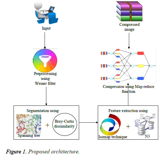
To overcome the drawbacks of lossless image compression an efficient approach known as Hadoop based image compression is proposed for seeking accurate image compression. Before the process of compression there are three major steps involved here. The first phase performs preprocessing for the given input image for the removal of noise and image blurring by the employment of Weiner filter. Weiner filter is different from other filter and has the special benefit of performing inverse filtering and controls output error. The output image from the Weiner filter is used as input to the Minimum Spanning Tree (MST) to segment the images and the MST segmentation is modified with the Bray-Curtis Dissimilarity (BCD) distance method which is a dimension independent distance. The advantage of using MST is that it segments the image based on the weights, so that efficient segmentation result can be obtained. After that BCD distance method is exploited to measure the dissimilarity between images. As a result it acquires accurate segmented image and this image is given as the input for the next phase. The next phase is the feature extraction. Here, Isomap technique with N3 (Non-parametric non-uniform intensity normalization) is used to extract the feature textures and intensity which will remove the extra information and minimize the image. Isomap technique is utilized for the purpose of reducing dimensionality which transforms high dimensional space to less space and N3 is a type of normalization technique in which the accurate needed information is extracted. The extracted dimensionally reduced features are compressed by performing compression technique with Hadoop based on Map Reduce function and is carried out to improve the encoding speed. The tools employed for processing in Hadoop is basically located in same servers, due to this the processing time will be reduced and security is cent percent guaranteed in Hadoop map reduce because it works with HDFS and HBase security that allows only approved users to operate on data stored in the system. Thus through this approach we can attain the efficient result. The process flow diagram of the proposed method is shown in the following Figure 1.
Pre-processing using Weiner filter
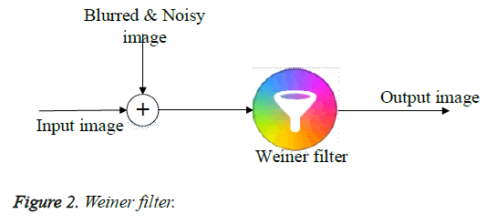
Pre-processing is the first step to be carried out in image processing. This is performed by the employment of Weiner filter in [26]. Weiner filter is different from other filter and has the speciality of performing inverse filtering and controls output error. In pre-processing phase, Weiner filter is employed to remove low frequency background noise and blurred image. Normally noise will appear due to malfunctioning pixels in camera sensors. In this paper Weiner Filter is utilized which is a type of linear filter. It is used to smoothen the image at low variance and high variance. When compared to linear filters, Weiner filter provides better results (Figure 2).
The inverse filtering is the restoration technique for deconvolution. At the point when the image is obscured by a known low pass filter, it is conceivable to get back the image by converse filtering. This converse filtering is exceptionally touchy to additive noise. The strategy for reducing one degradation at a time enables us to build up a restoration algorithm for each kind of degradation and just combine them. The Weiner filtering executes an ideal trade-off between converse filtering and noise smoothing. It expels the additive noise and modifies the obscuring in the meantime. The Weiner filtering is perfect as far as the mean square error. Weiner filter is utilized to limit the general mean square error in the process of backwards filtering and noise smoothing. The Weiner filtering is a linear estimation of the first Image. This depends on stochastic system. The output from the Weiner filter is the noiseless image.
Segmentation using Hybrid MST and BCD
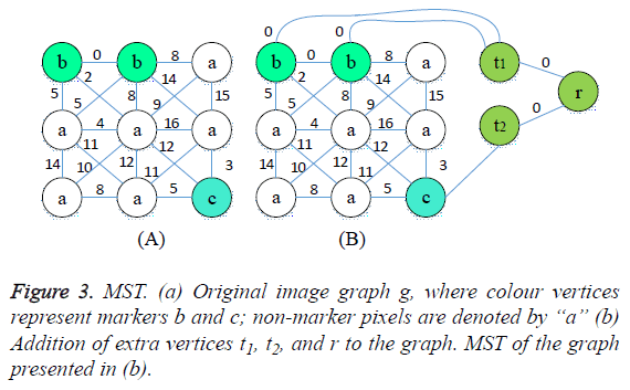
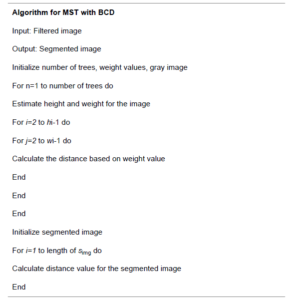
After the process of noise removal the next step is the segmentation of image. In this paper, MST method in [27] performs segmentation process. The advantage of using MST is that it segments the image based on weights, so that efficient segmentation results can be obtained. The main problem in MST is finding the minimum weight for set of edges that connects all their vertices when connected graph G with positive edge weights is given. Consider an image for this MST problem,
Undirected graph G=(V, E),
Where, V=the set of pixels,
E=the set of possible interconnections between pairs of pixels,
The weight of E is the difference of intensity values between neighbouring pixels. After that find an acyclic subset that connects all of the pixels and whose total weight is minimized. Eventually, the result of the segmentation is obtained by simply cutting edges whose weights are larger than a threshold value.
MST creation: The initial solution is a singleton set containing an edge with smallest weight and then current partial solution repeatedly expands by adding the next smallest weighted edge under constrain that no cycles are formed until no more edges can be added.
Steps for Mst generation
Input: A non-empty connected weighted graph with vertices V and edges E
Output: MST
Step 1: Initialize: Vnew={u}, where u is an arbitrary node from V, Enew={}
Step 2: Repeat until Vnew=V
Step 3: Select an edge {x, y} with minimal weight such that x is in Vnew and y
Step 4. Add y to Vnew and {x, y} to Enew
This above steps explains the creation of MST. The main reason behind using Prims algorithm is to construct MST that it tends to group pixels of similar (edges with small weights) together. If an image contains number of objects, each of which has a uniform depth, then the pixels representing each object will form a sub tree for the spanning tree obtained by Prims Algorithm. In general we would expect that if an image consists of number of objects represented by adjacent regions, Prims Algorithm would build a MST so that each object forms a sub tree. Along with the depth, height and width is taken into consideration so that, the objects will be grouped according to the depth. After the creation of adjacency graph, MST is to be constructed. MST is constructed to obtain shortest weight between points without removing the points in the point cloud. So creation of MST helps to find out all the points with minimum weight. At last an edge with largest weight is obtained as the final point. The output from the spanning tree will be segmented tree of image (Figure 3).
BCD: The segmented tree structured image which is the output from the MST is given as the input to the BCD method [28]. BCD is used to calculate the dissimilarity between images. Euclidean distance is one of the prevalent metric exploited to measure the distance between subjects. It makes use of principle of distance that is appropriate for univariate data. In literature, the other distance metrics are also appealing and that can be preferred for multivariate samples. Some of them still satisfy the basic axioms of what mathematicians call a metric, while others are not even metrics, but still make good sense as a measure of difference between two samples in the context of certain data. Among them, BCD metric is preferred that is popular in the study of environmental science problems. In ecology and science, the BCD metric is statistically used to quantify the compositional difference between two different destinations in view of counts at each site. With regards to ecological abundance, data collected from different inspecting locations quantifies the difference between tests utilizing Bray Curtis, which is one of the notable disparity metric. This measure gives off an impression of being sensible to achieve the results. Be that as it may, it doesn't fulfil the triangle disparity aphorism and hence is not a genuine distance when Bray and Curtis examine the Bray Curtis divergence metric. One of the suspicions of BCD metric is that the examples are taken from the same physical size such as area or volume. This is because uniqueness will be computed on crude counts not on relative counts as a result it leads to higher general abundance and is a piece of difference between these two samples that is, size and state of the count vectors will be considered in the metric. The computation includes summing the total differences between the counts and isolating this by the entirety of the abundances in the two samples. The general formula for calculating the BCD between two samples is given as follows.

Where, M is the dimensionality of the image, Y is the test image, X is the training image and Vnew, Enew are the ith values of the X and Y images to be compared. The Bray Curtis should be reversed for similarity computation is shown as below.
![]()
The classification performance of the LBP and ALBP methods are evaluated on face databases such as Extended Yale B, Yale A and our database.
The output after processing from MST and BCD is the best segmented image.
Feature extraction based on ISOMAP and N3
After the process of segmentation, the next phase is the feature extraction. In our proposed method, ISOMAP technique with N3 is employed to perform feature extraction. Iso map technique in [29] is utilized for the purpose of reducing dimensionality which transforms high dimensional space to less space and N3 [30] is a type of normalization technique in which the accurate needed information is extracted.
ISOMAP algorithm: The initial set is assumed as M real value vectors of high dimensional space Rh and is projected to low dimensional space Rl (l<h). The basic process of iso map is to obtain the expression of data set of observation space in a low dimensional space through distance preserving mapping when the distribution of data set possesses low dimensional embedding manifold structure. This algorithm is divided by the following steps.
Step 1: Form the neighbour graph G
Define with the Euclidean distance lBCD (Vnew, Enew) between points Vnew and Enew, if is located within the radius r of Vnew or among O nearest points of Vnew then connect Vnew and Enew points. And the length of the side equals to lBCD (Vnew, Enew)
Step 2: Calculate the shortest path
Calculate the shortest path lG (Vnew, Enew) between Vnew and Enew in the neighbour graph with Floyd algorithm and estimate the geodesic distance in topologic space p based on the said path.
Step 3: Form the l dimensional embedding
By adopting the classical MDS method, form a l dimensional embedding space X that keeps the essential structure of topologic space on distance matrix hG={lG (Vnew, Enew)}, hX is the Euclidean distance matrix of l dimensional space, coordinate vector is obtained through the following equations which can minimize error.
![]()
The matrix transform operator h=-HSH/2, D means distance matrix squared {DiVnew iEnew=h2 iVnew iEnew}, C means centralized matrix {CiVnew iEnew=DiVnew iEnew-1/m} the min value of Equation 9 is realized by acquiring the feature vector corresponding to d max feature values of matrix (hG).
ISOMAP gives the rules for determining the number of dimensionalities to be reduced and it defines the residual error e (l) to measure the error of dimensionality reduction.
![]()
Where R2 is linear correlation coefficient; generally, the higher the number of dimensionalities to be reduced the lower the residual error. ISOMAP determines the number of dimensionalities to be reduced in the following two situations:
1) Inflection point appears on the residual error curve
2) The residual error is small and approaches to certain threshold value.
One advantage of ISOMAP is that, for single manifold structure, “elbow” phenomenon appears when the variance of Equation 1 is solved during dimensionality reduction, based on this, the intrinsic dimensionality of manifold is judged.
N3 technique: In this phase, the intensity is corrected by using N3. And the problem of correcting intensity non-uniformity is simplified when it is modelled as a smooth multiplicative field. It is consistent with multiplicative non-uniformity arising from variations in the sensitivity of reception coil and with nonuniformity to a lesser extent due to induced currents and nonuniform excitation.
Consider the image formation in MR is
![]()
Where, y indicates the measured signal, x indicates the true signal emitted by the tissue, f is an unknown smoothly varying bias field, and e is white Gaussian noise assumed to be independent of x at location l. The problem of compensating for intensity non-uniformity is the task of estimating f.
In the noise-free case, the true intensities x at each voxel location i are independent identically distributed random variables. Using the notation ? (l)=log (y (l)) the image formation model becomes additive.
![]()
Let X, Y, F are the probability densities of x ?, ?, f ? respectively. Making the approximation that ? and f ? are independent or uncorrelated random variables, the distribution of their sum is found by the convolution as follows.

The non-uniformity distribution F can be viewed as blurring the intensity distribution J.
Correction strategy: From signal processing perspective, blurring due to the field reduces the high frequency components of Y. The task of correcting intensity nonuniformity is equal to that of restoring the frequency content of Y. Our approach for correcting the non-uniformity is to find the smooth, slowly varying, multiplicative field that maximizes the frequency content of Y. As evidence of the simple form of the distribution F, consider the distribution. These have been derived from the fields fitted to manually labelled regions of white matter on 12 individuals. Each individual was scanned using the same pulse sequences but on a different MR machine. As the large scale features of F vary little between scans. Returning to the optimization criterion, one could be in a principle search through all possible fields f ? to find the one that maximizes the high frequency content of Y.
There are two drawbacks arises in this approach, (i) large search space for 3D fields, (ii) computation of entropy is difficult.
In this approach, we propose a distribution for Y by sharpening the distribution X, and then to estimate corresponding smooth field which produces a distribution Y close to the proposed one. If F is Gaussian, then it searches only the space of all distributions Y corresponding to F with zero mean and given variance. In this way the space of all distributions Y is collapsed down to a single dimension in the width of the F distribution.
In practice, the field distribution F is only approximately Gaussian and some of our assumptions, such as zero noise, are violated. The benefit of this approach is that between subsequent estimates of Y, corresponding smooth field f ? is estimated. The constraint that the field be smooth changes the shape of the proposed distribution Y to the one that is consistent with the field. These iterations proceed until no further changes in f ? or X result from de-convolving narrow Gaussian distributions from X.
Field estimation: Further theory is presented here to explain the process of proposing distributions for Y and estimating corresponding fields. For notational simplicity, we will assume that the true distribution of intensities Y can be arrived at a single iteration by de-convolving a distribution F, which is Gaussian from X. The full iterative description of the method is left for a subsequent section.
For the given the distribution Y, the method for estimating corresponding field is as follows. For a measurement of x ? at some location l, ? is estimated using the distributions Y and F. Since the choice of the location l is arbitrary, the measurement x ? can be treated as a random sample from the distribution X. The expected value of ? gives the measurement x ? as follows.

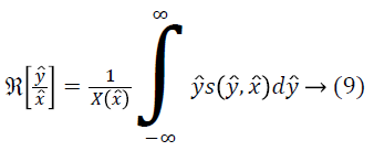
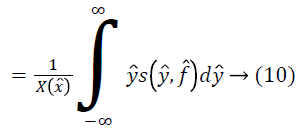
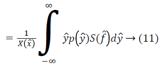
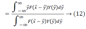
An estimate of f ? can be obtained using the estimate of from Equation 17 as follows.

Where, f ?e is an estimate of f ? at location l based on the single measurement of x ? at l. This estimate can be smoothed by the operator Sm to produce

An estimate of f ? based on all of the measurements in a neighborhood of l.
Given a distribution F and the measured distribution of intensities X, the distribution Y can be estimated using a deconvolution filter as follows:

![]()
Where, * denotes complex conjugate, F ? is the Fourier transform of F, and μ is a constant term to limit the magnitude of G ?. This estimate of Y is then used to estimate a corresponding field f ?.
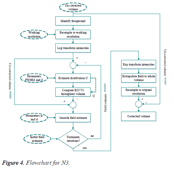
Implementation details: The nonparametric correction process is shown in the Figure 4. Besides the processing steps described previously, there are number of steps needed for practical implementation of the algorithm.
Here ellipses represents user-selected parameters and priors. Rectangles are processing steps. The flow of volumetric data and other data is represented by solid lines and dashed lines. Circles perform arithmetic operations on a voxel by voxel basis. The result of the process is a corrected volume.
The first step “identify foreground,” is to segment and remove empty regions from the volume. Besides the numerical problems associated with transforming values near zero to the log domain, these background regions provide no information about the non-uniformity field. Since the accuracy of this segmentation is not critical, the foreground is determined using a simple threshold chosen automatically by analysing the histogram of the volume.
A histogram with equal-size bins and a triangular Parzen window is used to estimate X. Given a set of N measurements x?(lu) and locations lu, X, is estimated as follows:


Where, x? v is the centers of the bins and dis the distance between them. For a typical 20% bias field, the scale factor f ranges from 0.9 to 1.1 which corresponds to f ? between 0.1 and 0.1. MR volumes generally have sufficient data to estimate X at a resolution d better than a tenth of this range.
Smoothing the non-uniformity field at full resolution is computationally expensive, so the MR data is sub sampled without averaging to a lower resolution. Since the nonuniformity field is slowly varying, a 1 mm iso-tropically sampled volume is reduced to 3 mm and has a negligible effect on the field estimate and substantially accelerates computation. The processing of volume with ten iterations of N3 method is reduced from 4.5 h to 7 min of CPU time on a 200 MHz Intel Pentium workstation running Linux by re sampling to the coarser resolution. The final field estimate is re sampled to the original resolution and used to correct the original volume. The measure used to terminate the iterations is computed as follows:

Where, cn is the ratio between subsequent field estimates at nth location, ϑ denotes standard deviation, and ρ denotes mean. This measure is chosen so as to be insensitive to global scale factors that may accumulate with iterations. Iteration is stopped when e drops below 0.001, typically after ten iterations.
Smoothing: The manner in which the field estimate is smoothed has significant impact on the performance of the correction method. Smoothing is particularly challenging for this problem because the scale over which the field varies is compared to the size of the region being smoothed. Conventional filtering techniques proved unsatisfactory for this application since boundary effects significantly degraded overall performance.
The smoothness of the approximation is determined by two parameters: ω is the smoothing parameter and d is the distance between basis functions. Since splines are being used as filter for this application, the smoothness of the approximation must be chosen rather than derived from the data. The relationship between the smoothness of the approximation and the smoothing parameter is nonlinear. However, the normalization of the Bsp line has been chosed to eliminate the dependence of ω on scale and number of data points ω, can be fixed and the distance between basis functions varied instead. The output from this hybrid technique will be optimal extracted features.
Compression based on Hadoop map reduce
After the process of feature extraction, compression is the final step. This is done by the utilization of Hadoop map reduce [31]. The tools employed for processing in Hadoop is basically located in same servers, due to this the processing time will be reduced and security is cent percent guaranteed in Hadoop map reduce because it works with HDFS and H Base security that allows only approved users to operate on data stored in the system.
HADOOP: It is an open source framework used to process big data or datasets in a distributed environment. It provides with huge data storage space and excessive processing power. In our proposed scheme the compression process is done by Hadoop based on map reduce function. It is used to improve the encoding speed.
Map reduce: Map Reduce is used to process the data stored within Hadoop File System. Here the output is in the form of a <key, value>pair. A map reduce program consists of following 3 parts:
1. Mapper
2. Reducer
3. Record writer
Mapper: The text line input is divided in the form of no of input splits. The mapper process the data i.e., Input splits. Each of these input splits are assigned to a mapper.
No of input splits=No of mapper
The mapper doesn’t accept text line input. It allows the input to be in a key, value pair. To convert the text line input to<key, value> pair, record reader is used. The record reader converts the byte oriented input into record oriented input.
Reducer: It obtains sorted<key, value>pairs sorted by the key. The value list contains all the values with the same key produced by mappers. Reducer combines the output from all the mappers and generates the final output. This final output shouldn’t have any duplicate keys.
Record writer: Record writer writes the output to the output file by converting into text line-form.
Steps for Hadoop mapreduce
Step 1: Map (key, value):
{
It takes set of large data and processes it to give output in form of smaller chunks. It takes file from Hadoop distributed
File system and input is processed line by line.
For each attribute:
Output index and its value and class label of instance to generate key value pairs.
Return output key and output value
}
Step 2: Reduce (key, value)
{
Count occurrences of combination: attribute index and its value and class Label.
Print count against each combination.
}
The output from the Hadoop map reduction will be the compressed feature after encoding.
Results
The following table contains the information about the values obtained during implementation (Table 1).
| Name | 'en_val' |
|---|---|
| Global | 0 |
| Sparse | 0 |
| Complex | 0 |
| Persistent | 0 |
| Nesting | (1 × 1 struct) |
| Bytes | 3840 |
| Size | (16 30) |
| Class | 'double' |
| Encryption time | 0.11097 s |
| Decryption time | 0.10745 s |
| PSNR value | 2.0108 |
| Bit Rate | 1 |
| Compression ratio | 33.584616 |
Table 1: Meta data information.
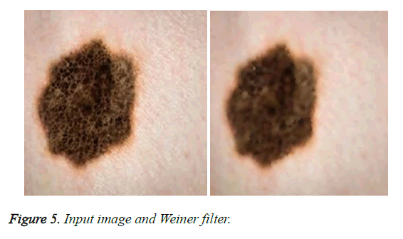
This section shows the performance of the proposed Hadoop based image compression and the results obtained by them. In our proposed system the main objective is to accurately compress the given input image and overcome the problems that occur during image compression. The input contains some noise and this noise is removed by means of Weiner filter. The difference between input image and noiseless image is shown below in Figure 5.
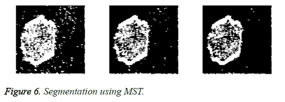
After the removal of noise the first stage should be done in image processing is the segmentation of image. Here hybrid technique namely MST with BCD is employed for the purpose of segmentation. The segmented image using MST is shown below in Figure 6.
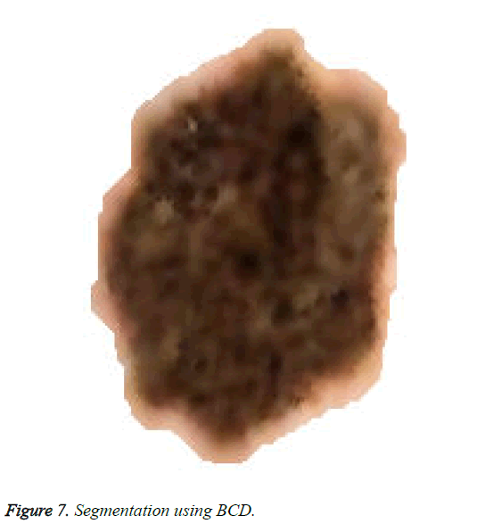
The segmented image after applying BCD is shown below in Figure 7.
After the process of segmentation the next step is the feature extraction. Here the process of extraction of feature is done by means of isomap technique and N3 (normalization technique). The features after the process of extraction is compressed and encrypted by the employment of Hadoop map reduce. The compressed image is shown in Figure 8.
Performance result for the proposed approach
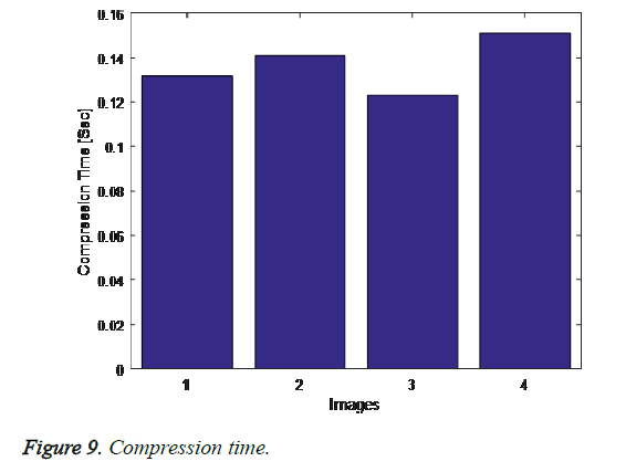
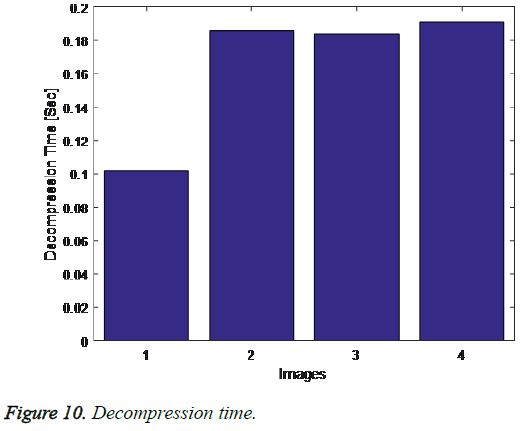
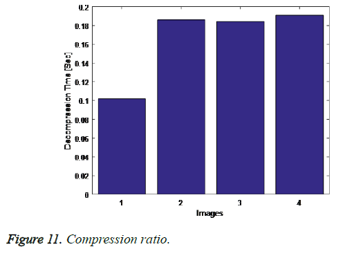
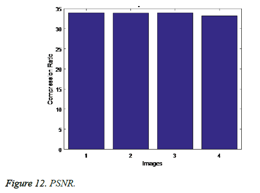
The following graph shows the results of our proposed approach via the parameters compression time, decompression time, compression ratio and PSNR (Figures 9-12).
Comparison result
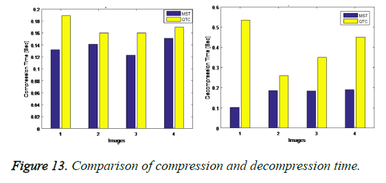
The compression time and decompression time must always be low for obtaining efficient result. The compression and decompression time is compared with the existing QTC approach is shown below in Figure 13.
To evaluate the compression result two measures are commonly applied. The first one is the PSNR (peak signal to noise ratio) and the next is the CR (Compression Ratio).
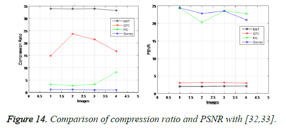
The compression ratio for the compressed image must be always high in order to obtain good quality image. Compression is nothing but it eliminates unwanted information in order to gain high compression ratio. The compression ratio for our proposed system compared with the existing FIC approach, QTC and survey is shown below in Figure 14. PSNR is the process of measuring the quality of reconstructed image. PSNR value for accurate compressed image must be always low. The PSNR value for our proposed system compared with the existing FIC approach, QTC and survey is shown below in Figure 14.
Conclusion
In image compression, the problem that occurs is the low image quality, compression ratio and speed. To solve and overwhelm these issues, Hadoop based image compression approach is proposed in this paper. The comparison results are obtained for the parameters compression time, decompression time, compression ratio and PSNR. The comparison tables and the graphs illustrated the performance of the proposed method with other researches. Hence with the aid of this proposed technique the problems in the existing image compression are reduced to greater extends.
References
- Zhou N, Aidi Z, Fen Z, Lihua G. Novel image compression–encryption hybrid algorithm based on key-controlled measurement matrix in compressive sensing. Opt Laser Technol 2014; 62: 152-160.
- Padmavati S, Vaibhar M. DCT combined with fractal quadtree decomposition and Huffman coding for image compression. Condition Assessment Techniques in Electrical Systems (CATCON) 2015; 28-33.
- Bansal N. Image compression using hybrid transform technique. J Glob Res Comp Sci 2013; 4: 13-17.
- Kamisli F. Block-based spatial prediction and transforms based on 2D Markov processes for image and video compression. IEEE Trans Imag Proc 2015; 24: 1247-1260.
- Rufai AM, Gholamreza A, Hasan D. Lossy image compression using singular value decomposition and wavelet difference reduction. Dig Sig Proc 2014; 24: 117-123.
- Xiao B, Gang L, Yanhong Z, Weisheng L, Guoyin W. Lossless image compression based on integer discrete tchebichef transform. Neuro Comput 2016; 214: 587-593.
- Belloulata K, Amina B, Shiping Z. Object-based stereo video compression using fractals and shape-adaptive DCT. AEU Int J Electron Commun 2014; 68: 687-697.
- Wu CP, Kuo CC. Design of integrated multimedia compression and encryption systems. IEEE Trans Multimed 2005; 7: 828-839.
- Cheng H, Li X. Partial encryption of compressed images and videos. IEEE Trans Sig Proc 2000; 48: 2439-2451.
- Ibrahim RA, Sherin YM, Saleh ME. An enhanced fractal image compression integrating quantized quadtrees and entropy coding. Innovations in Information Technology (IIT). Proceedings of 11th International Conference IEEE 2015: 190-195.
- Zhou N, Aidi Z, Fen Z, Lihua G. Novel image compression–encryption hybrid algorithm based on key-controlled measurement matrix in compressive sensing. Opt Laser Technol 2014; 62: 152-160.
- Song, C, Sud S, Madjid Mi, A robust region-adaptive dual image watermarking technique. J Vis Commun Imag Represent 2012; 23: 549-568.
- Potluri US, Arjuna M, Renato CJ, Fabio BM, Sunera K, Amila E. Improved 8-point approximate DCT for image and video compression requiring only 14 additions. IEEE Trans Circ Sys I Regular Papers 2014; 61: 1727-1740.
- Bairagi VK, Sapkal AM. Automated region-based hybrid compression for digital imaging and communications in medicine magnetic resonance imaging images for telemedicine applications. IET Sci Measure Technol 2012; 6: 247-253.
- Rawat C, Sukadev M. A hybrid image compression scheme using dct and fractal image compression. Int Arab J Inf Technol 2013; 10: 553-562.
- Lin YH, Ja LW. Quality assessment of stereoscopic 3D image compression by binocular integration behaviors. IEEE Trans Imag Proc 2015; 23: 1527-1542.
- Qin C, Chin-Chen C, Yi-Ping C, A novel joint data-hiding and compression scheme based on SMVQ and image in painting. IEEE Trans Imag Proc 2014; 23: 969-978.
- Zhang X. Lossy compression and iterative reconstruction for encrypted image. IEEE Trans Info Forens Secur 2011; 6: 53-58.
- Karri C, Umaranjan J. Fast vector quantization using a Bat algorithm for image compression. Eng Sci Technol Int J 2016; 19: 769-781.
- Kumar G, Pragati S, Scholar PG. A survey of various image compression techniques for RGB images. InT j Eng Sci 2016; 4905.
- Zhang X, Ren Y, Shen L, Qian Z, Feng G. Compressing encrypted images with auxiliary information. IEEE Trans Multimed 2014; 16: 1327-1336.
- Chaurasia V, Vaishali C. Statistical feature extraction based technique for fast fractal image compression. J Vis Commun Image Represent 2016; 41: 87-95.
- Dar Y, Bruckstein AM, Elad M, Giryes R. Postprocessing of compressed images via sequential denoising. IEEE Trans Image Process 2016; 25: 3044-3058.
- Hussain AJ, Dhiya AJ, Naeem R, Paulo L. Hybrid neural network predictive-wavelet image compression system. Neuro Comput 2015; 151: 975-984.
- Wu MS. Genetic algorithm based on discrete wavelet transformation for fractal image compression. J Vis Commun Image Represent 2014; 25: 1835-1841.
- MalothuNagu NV. Image de-noising by using median filter and weiner filter. Int J Innov Res Comp Commun Eng 2014; 2.
- Geetha M, Rakendu R. An improved method for segmentation of point cloud using minimum spanning tree. Communications and Signal Processing (ICCSP). proceedings of IEEE International Conference 2014; 833-837.
- Shyam R, Singh YN. Evaluation of eigen faces and fisher faces using bray Curtis dissimilarity metric. In Industrial and Information Systems (ICIIS). Proc Int Conf 2014; 1-6.
- Xu XL, Chen T. ISOMAP algorithm-based feature extraction for electromechanical equipment fault prediction. Image Sig Proc CISP09 2nd International Congress IEEE 2009; 1-4.
- Sled JG, Zijdenbos AP, Evans AC. A nonparametric method for automatic correction of intensity nonuniformity in MRI data. IEEE Trans Med Imaging 1998; 17: 87-97.
- Desai S, Roy S, Patel B, Purandare S, Kucheria M. Very Fast Decision Tree (VFDT) algorithm on Hadoop. Comp Commun Contr Autom (ICCUBEA) Proc IEEE Int Conf 2016; 1-7.
- Chaudhari RE Dhok SB. Wavelet transformed based fast fractal image compression. Circ Sys Commun Info Technol Appl 2014; 2014: 65-69.
- Bhavani S, Thanushkodi K. A survey on coding algorithms in medical image compression. Int J Comp Sci Eng 2010; 2: 1429-1434.
