Biomedical Research

Abstract

In Magnetic Resonance Imaging (MRI), the information about the image is collected in the form of Radio Frequency (RF) signals with a range of frequencies and phases. The MR image is then reconstructed by performing the inverse Fourier Transform of the acquired raw data (k-space). A good understanding of the k-space offers important insight into the basic properties related to signal-to-noise ratio, image distortion, resolution and contrast in MRI. This paper presents an implementation of various MATLAB functions for exploring the different properties of k-space such as acceleration factor, filtering schemes, different kinds of artefacts, quantifying parameters. The user is also able to visualize different kinds of trajectories (Cartesian and Non-Cartesian) using animations. The main purpose of this toolbox is to present an interactive graphical user interface (GUI) using MATLAB for researchers and graduate/undergraduate students to develop better understanding of MRI. In order to evaluate the usefulness of the tool, it is used by graduate/undergraduate students in different projects. It has been observed that the students were able to use the toolbox “k-space and Interactive Educational Tool” effectively without prior background knowledge in k-space. The software toolbox is available for free download from our research group website.

Keywords

k-space, MRI, Image reconstruction techniques

Introduction

Biomedical Engineering emerged as a new discipline that addresses the challenges in developing advanced tools to improve healthcare diagnosis and treatment [1,2]. This discipline involves the study of anatomy and physiology through the use of medical imagery, such as ultrasound, computerized tomography (CT), and MRI. Medical imaging is in fact a discipline on its own which involves the use of technology to capture images from the inside of the human body which are widely used as diagnostic and teaching tools.

Magnetic Resonance Imaging (MRI) is a non-invasive imaging modality to have an insight into the human body. In MRI the object to be imaged is placed in a strong magnetic field, known as Bo field, and a Radio Frequency (RF) signal (42.58 MHzT^-1), called B1 field, is applied to selectively excite the parts of the object to be imaged. The signals from the excited slices of the object are obtained using receiver coils. The data received from these receiver coils is stored in k-space (raw data space of MRI) [3]. The inverse Fourier transform of the kspace provides the Magnetic Resonance (MR) image.

The authors are able to find only one educational tool available in the literature that focuses on k-space simulation is an MRI educational tools using MATLAB Simulink in which the user can modify several parameters in k-space and visualize the effects on the reconstructed image [4]. However this toolbox only deals with the effects of rectilinear trajectory on k-space [3]. Other major limitations of the toolbox include the absence of radial and spiral trajectory, animated effects of different trajectories, absence of important quantifying parameters e.g. artefact power of the reconstructed image, missing effects of rotating/flipping the k-space parameter, missing effects of zero padding in the under-sampled k-space and the image reconstruction from the non-rectilinear trajectories.

The aim of this paper is to present an interactive graphical user interface (GUI) that provides an immediate insight into the theoretical aspects of k-space in MRI. An introduction to the kspace is given below in Section II. Section III describes the design and structure of the developed software. Section IV describes the functionality of the software. Finally the paper is concluded. . The software toolbox is available for free download from our research group website [1].

Basics

What is k-space?

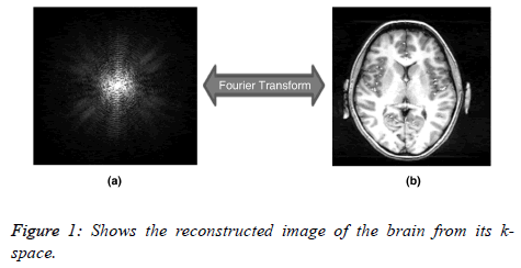
MRI works by acquiring signals from the Hydrogen nuclei in the object under observation. The object to be scanned is placed in a strong magnetic field known as B_o field, which causes the spins of the hydrogen nuclei to align either parallel or anti-parallel to the field. Radio frequency (RF) pulse, called B₁ field is then applied to excite the Hydrogen nuclei. Receiver coils are then used to receive the signals from these excited nuclei. The acquired signals are stored in k-space (raw data space of MRI). The k-space represents the locations of the acquired signals which have been encoded with frequency and phase encoding along the x and y directions. As multiple frequency encoded echoes are collected with different phaseencoding gradients, (they are placed as horizontal lines in the corresponding k-space with the vertical direction representing the phase-encoding gradient values or otherwise. Figure 1 shows the k-space and its associated image.

Figure 1. Shows the reconstructed image of the brain from its kspace.

Why it is called k-space?

The Fourier series describes a given function as infinite linear combinations of stationary plane waves, each of which may be characterized by an amplitude and a wave number. The term wave number refers to the number of complete wave cycles that exist in one meter of linear space. The wave number is traditionally denoted by the letter “k” [5]. Three different gradient fields are used in MRI usually called G_x, G_y and G_z. These three gradient components are the three coordinates and actually define a domain, or more colloquially a “space” which we have come to call k-space [5]. The choice of a letter “k” is based on a tradition among physicists and mathematicians to use that letter to stand for spatial frequency in other similar equations (e.g. equations that describe the propagation of light, sound or radio waves).

How k-space data is formed?

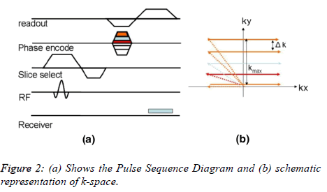
Figure 2 shows a simple example of Pulse Sequence Diagram (PSD) [6] that illustrates the sequence of events that occur during MRI data acquisition. Different types of pulse sequence diagram are discussed in the literature [7]. The PSD shows (Figure 2) the timings of RF pulse, gradient fields and the data acquisition. An RF pulse is applied initially along with a slice selective gradient (Figure 2a). This is followed by the phase encoding gradient (G_PE). Finally a readout (Frequency Encoding) gradient (G_FE) is applied and the MR signal is collected. In order to fully acquire the k-space data, this sequence needs to be repeated for every new line of k-space, the only difference each time will be a step-wise increment in the phase encode gradient. Once the full k-space data is acquired, its inverse Fourier transform (iFFT) provides an MR image. It is important to note that the number of Phase Encode (PE) steps define how many times a pulse sequence needs to be repeated which results in long MRI scan time. K-space represents how much and how long the gradients are turned on if the applied phase encode gradient is zero, it takes us to the left of the k-space and the readout gradient will fill a line by sweeping across the k-space (Figure 2b). When phase encoding gradient is applied, it shifts the readout line in k-space along the phase encode direction by an amount . The magnitude of is inversely proportional to the Field of View (FOV).

Figure 2. (a) Shows the Pulse Sequence Diagram and (b) schematic representation of k-space.

The number of PE steps has a direct effect on the scan time which can be minimized by reducing the number of PE steps. Equation 1 defines the different parameters which affect scan time in MRI (for line by line acquisition of k-space data only) where (Repetition time) is the time between the application of an excitation pulse and the application of the next pulse and is measured in milliseconds, is the number of signal averages and N_PE is the number of PE lines [8]. However reducing the number of PE lines produces aliased images [9].

Scan Time=TR*NSA*N_PE (1)

Properties of k-space

The size of the k-space is the same as the size of the MR image e.g. both may be 256 × 256. However a point in the k-space does not correspond to a point in the image matrix [5]. The data at the center of the k-space contains most of the signal information and the contrast information of the image, and the data along the outer edges contains information about the edges and boundaries. Another important property of k-space is the existence of symmetrical data; according to this property only half of the k-space data will need to be collected and the remaining half of the k-space can be estimated mathematically by using complex conjugate synthesis. This can potentially reduce the MR data acquisition time by approximately ; unfortunately it reduces the SNR by a factor of √2 [10,11].

To further improve the spatial resolution of the MR image it may be a good idea to acquire just over half of the data in kspace. These techniques have been used in the past to reduce the MR scan time but did not provide successful results because of low SNR values of the reconstructed image [12].

Results

In order to speed up the MR data acquisition, either the k-space data must be collected at a faster pace by reducing the (pulse repetition time) (Equation 1) which may not be possible because of the physiological limits [13]. Actually this requires rapid switching of the magnetic field gradients which may induce electrical currents in the patient, potentially causing peripheral nerve stimulation [14]. Another approach to decrease the MR scan time is to reduce the amount of the kspace data collected i.e. must be reduced but it leads to the aliasing artefacts [9,15]. Aliasing artifacts become more apparent if more PE lines are skipped in the k-space. In order to remove this aliasing, considerable efforts have been made in the recent past to develop optimized parallel imaging algorithms [16]; which are beyond the scope of this paper.

Software Structure and Design

The proposed tutorial “k-space an Interactive Educational Tool” has been developed using MATLAB 2013a. The main purpose of this tutorial is to develop an education toolbox that will demonstrate the k-space and its effects on the associated image. In this toolbox the user is able to visualize the effects on the reconstructed image by varying different parameter(s) in k-space e.g. acceleration factor, white pixel effects, filtering schemes (low pass filter, high pass filters and band-pass filters), applying rotation or flipping the data in k-space and its effect on the reconstructed image and gridding effects on NC (non-Cartesian) trajectories. The user is also able to visualize and animate the different gradient waveforms (rectilinear and spiral etc.). Furthermore the user can compare the images (e.g. original and the reconstructed images) by the help of quantifying parameters e.g. Artefact Power [17], SNR [18] and image reconstruction time.

All the experiments performed to test this software used the data acquired from a healthy volunteer (human head MR transversal slice data). This data was acquired at St Mary’s Hospital London using a steady state gradient echo sequence with 256 × 256 image grid having the following parameters: TE=10 msec, TR=500 msec, FOV=20 cm, Bandwidth=31.25 KHz, Slice Thickness=3 mm, and Flip Angle=50 degrees. However the user is not restricted to use this k-space data only, this educational toolbox allows the user to load any square kspace image data having size less than or equal to 512 × 512.

This interactive GUI consists of three main MATLAB windows. The interaction between these independent windows is realized using MATLAB global variables which are available to all the functions within a MATLAB session. At the startup MATLAB stores all the references of the GUI objects in a specific variable. By declaring a global variable holding a copy of the references to GUI objects of the figure, the GUI objects can be accessed from any function in the program. To keep track of the numerous references every MATLAB figure (e.g. Visualize Trajectories, Cartesian Data and Non-Cartesian Data) creates its own global variable. The proposed toolbox is split into three main parts:

• Visualize Trajectories: visualize and animate different kspace trajectories (e.g. Cartesian and Spiral)

• Cartesian Data: The effects on the reconstructed image can be observed by varying different parameters of Cartesian data e.g. acceleration factor, different filtering schemes etc.

• Non-Cartesian Data: The effects of varying different parameters of Non-Cartesian data e.g. acceleration factor on the reconstructed image can be seen.

Operation of the Software

The main purpose of this toolbox is to show clearly how the raw data is filled in k-space by exploring different trajectories, how the MR image is reconstructed from the k-space, how aliasing artefacts are created, what quantifying parameters can be used to analyze the reconstructed image.

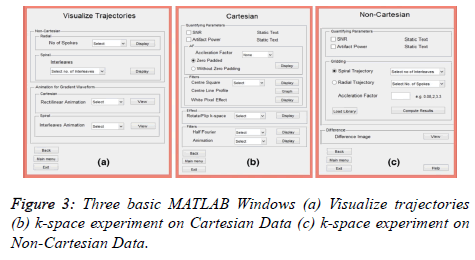
The primary three MATLAB Windows (Figure 3) defined the functionality of visualizing trajectories, Cartesian data and Non-Cartesian data. The main features of each MATLAB window are discussed below.

Figure 3. Three basic MATLAB Windows (a) Visualize trajectories (b) k-space experiment on Cartesian Data (c) k-space experiment on Non-Cartesian Data.

Visualize trajectories

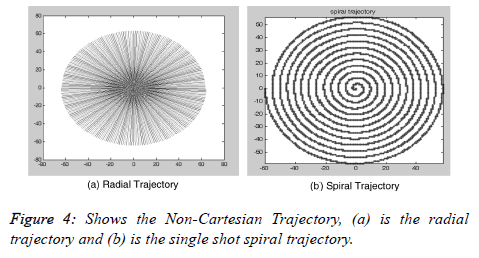
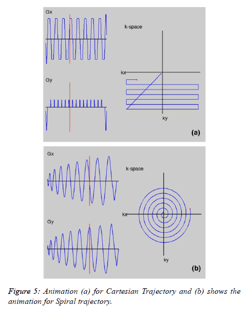
Figure 3a shows the MATLAB window for Visualize Trajectory. The user can visualize different trajectories (e.g. Radial and Spiral) not only for different acceleration factors but also by varying the number of spokes in radial and the number of interleaves in the spiral trajectory. Figure 4a shows the radial and Figure 4b shows the spiral trajectory masks. The “Visualize Trajectory” MATLAB window (Figure 3a) also loads the gradient waveforms showing the animation of traversing only 16 lines (Rectilinear trajectory) in k-space (far fewer than the actual experiment). Figure 5a shows the animation for Cartesian trajectory. The main purpose of showing this animation is to familiarize the user for the direction of the phase encoding and frequency encoding. The user can also visualize the x-axis traversing or y-axis traversing.

Figure 4. Shows the Non-Cartesian Trajectory, (a) is the radial trajectory and (b) is the single shot spiral trajectory.

Figure 5. Animation (a) for Cartesian Trajectory and (b) shows the animation for Spiral trajectory.

The user can also investigate the following effects from this animation:

• and axis are independent i.e. the current location along k_x is determined solely by the waveform, and that of k_y by

• Along a given direction, the sign of the waveform determines whether the trajectory is traversed in a positive or negative direction

• The user can visualize the spiral trajectory which is formed by a complex gradient waveform. Figure 5b provides a sketch of the animation of spiral trajectory.

Cartesian data

Mostly, clinical MR imaging is performed by acquiring kspace data along a Cartesian or rectilinear trajectory where the data is sampled line-by-line on a rectangular grid. A benefit of this sampling trajectory is that the data is uniformly sampled and the images can be reconstructed using FFT. In this window of the proposed toolbox, the user can visualize the effect on the image and its field-of-view by varying different parameters such as acceleration factor, filtering schemes and quantifying parameters. Beside that the user can visualize the effect of filtering schemes with the help of the animations.

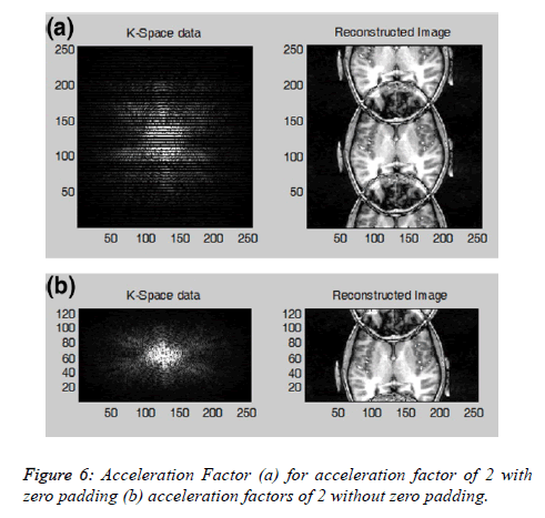
Acceleration factor: In Cartesian data the number of PE steps can be reduced by a reduction factor R (or acceleration factor) by increasing the distance between the equidistantly sampled k-space lines, resulting in an increased imaging speed. If every other line in the k-space is acquired, the MR data acquisition is accelerated by a factor R=2. The reduction of PE steps is also known as sub-sampling. This sub-sampling of the k-space yields a reduced Field of View (FOV) in the PE direction associated with the fold-over artifacts, as shown in Figure 6. The user can further explore the effect of filtering schemes on the reconstructed image by enabling the option “zero padded” (when the skipped line of the k-space is filled with zeros) and without zero padding (when the skipped k-space lines are deleted). Figure 6a shows the k-space and the reconstructed image with the zero padded data and Figure 6b shows the kspace and the reconstructed image without zero padding.

Figure 6. Acceleration Factor (a) for acceleration factor of 2 with zero padding (b) acceleration factors of 2 without zero padding.

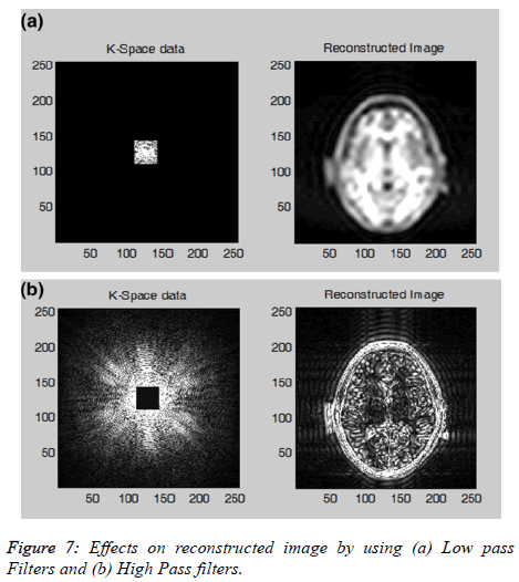
Filtering scheme: The user will be able to apply low, high, and band-pass filtering schemes on k-space data to visualize the effect on the image. The data at the center of the k-space contains mostly the signal and contrast information of the image, and the data along the outer edges contains all the information about the edges and boundaries. Figure 7a shows the effect on the reconstructed image by selecting the central kspace data only and Figure 7b shows the effects on the reconstructed image by selecting the outer boundary of the kspace.

Figure 7. Effects on reconstructed image by using (a) Low pass Filters and (b) High Pass filters.

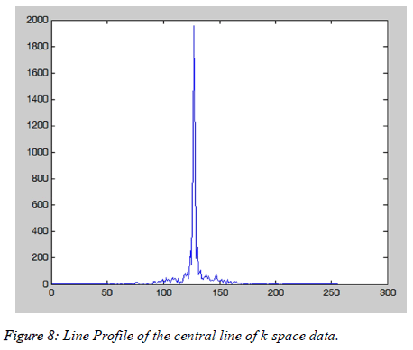
The Cartesian Trajectory MATLAB windows (Figure 8) also provide the information about the line profile of the central line of the k-space (Figure 9). White pixel effect is when a single or few values in the k-space data points are replaced with zero(s) or one(s). This causes the dark stripes overlaid on the image as shown in the Figure 9. This changing of the single value in kspace shows that a point in k-space does not correspond to the same location in image. The user can visualize the white pixel effect on any k-space data location by interactively altering a value in the k space.

Figure 8. Line Profile of the central line of k-space data.

Figure 9. White pixel effect in the form of dark strip appear on the reconstructed image.

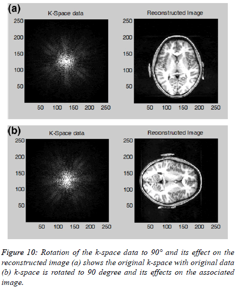
The reconstructed image is rotated or flipped if the k-space is transformed accordingly. The user can also transform; rotate (90°, 180° or 270°) or flip (horizontal or vertical) the k-space data and see the rotated or flipped effects on the reconstructed image as shown in the Figure 10. Another important property of the k-space is the existence of symmetrical data; according to this property only half of the k-space data will need to be collected and the remaining half of the k-space can be estimated mathematically by using complex conjugate synthesis; this process is known as Half Fourier. This can potentially reduce the MR data acquisition time by approximately ; unfortunately it reduces the SNR by a factor of [10]. The user can visualize the Half Fourier k-space data and its effects on the reconstructed image. The user can further explore this option (Half Fourier) by varying the Half Fourier parameters e.g. selecting some extra (more than half of the kspace data lines) PE lines and its effects on the reconstructed image.

Figure 10. Rotation of the k-space data to 90° and its effect on the reconstructed image (a) shows the original k-space with original data (b) k-space is rotated to 90 degree and its effects on the associated image.

Animation: The user can visualize the animated effect on the reconstructed image by gradually increasing or decreasing the size of the central k-space window. Different animation effects are “low pass filter to high pass filter” and similarly from “high pass filter to low pass filter.”

Quantifying parameter (Artefact power, SNR and Image reconstruction time) can be used to test the quality of the reconstructed images.

Non-cartesian data (NC)

In NC MRI, the k-space data is not collected along the parallel rows but instead along the trajectories such as radial or spiral as seen in Figure 4. The main advantages of using NC trajectories are: continuous repeated sampling of the center of the k-space, an efficient k-space coverage and intrinsic motion correction [13]. On the other hand, Fast Fourier Transform (FFT) cannot be applied directly on the acquired NC trajectory based k-space data. This NC trajectory based k-space data is first re-sampled onto a rectilinear grid by using Gridding [19] and then an inverse FFT is performed on the re-sampled data to reconstruct an MRI image. The same procedure is followed in this GUI interface; in non-Cartesian MATLAB window the user has the flexibility to choose the desired parameters for NC trajectories (radial or spiral) by varying the acceleration factor, number of spokes in radial trajectory and number of interleaves in spiral trajectories as shown in Figure 3c. The user can also see the difference of the original and reconstructed image (using iFFT) by enabling the option of “difference image” which shows the image difference between the original image and the reconstructed image.

Conclusion

This wizard based interactive tool provides a platform for the students and beginners who want to explore different aspects of k-space for MR image extraction. This toolbox provides interactive interface, specifically designed for educational purposes, which allows a much more intuitive and fast learning. Three different datasets (stomach, brain and knee) have been provided with this toolbox. The user is able to test any kind of k-space dataset in this tutorial. Future work will be to introduce more plugins and features after getting feedback from the current users. This toolbox can be obtained by reaching at the institutional web page address or by contacting the author at mehmoodqureshi@comsats.edu.pk.

References

1. Qureshi M, Shahid AR, Kaleem M, Omer H. Journey through k-space.
2. Enderle JD, Bronzino JD. Introduction to biomedical engineering. Academic Press 2012.
3. McRobbie DW, Moore EA, Graves MJ, Prince MR. MRI from Picture to Proton: Cambridge University Press, 2006.
4. Moratal DA, Vallés-Luch L, Martí-Bonmatí, Brummer ME. k-Space tutorial: an MRI educational tool for a better understanding of k-space. Biomed Imag and Interv J 2008 4.
5. Mezrich R. A perspective on K-space. Radiology 1995; 195: 297-315.
6. Weishaupt D, Froehlich J, Nanz D, Köchli VD, Pruessmann K, Marincek B. How does MRI work? an introduction to the physics and function of magnetic resonance imaging. Springer 2008.
7. Hennig J. K-space sampling strategies. European radiology 1999; 9: 1020-1031.
8. Hashemi RH, Bradley WG, Lisanti CJ. MRI: the basics: Lippincott Williams & Wilkins, 2012.
9. Haacke EM, Brown RW, Thompson MR, Venkatesan R. Magnetic resonance imaging. Phys Princpl Seq Des 1999.
10. Pauly J. Non-cartesian reconstruction 2007; 7.
11. Bernstein MA, King KF, Zhou XJ. Handbook of MRI pulse sequences: Elsevier, 2004.
12. Schoenberg SO, Baert A, Dietrich O, Reiser MF. Parallel imaging in clinical MR applications: Springer, 2007.
13. Wright KL, Hamilton JI, Griswold MA, Gulani V, Seiberlich N. Non-Cartesian parallel imaging reconstruction. J Mag Res Imag 2014.
14. Vogt FM, Ladd ME, Hunold P, Mateiescu S, Hebrank FX. ncreased time rate of change of gradient fields: effect on peripheral nerve stimulation at clinical MR imaging. Radiology 2004; 233: 548-554.
15. Morelli JN, Runge VM, Ai F, Attenberger U, Vu L, Schmeets SH. An image-based approach to understanding the physics of MR artifacts. Radiographics 2011; 31: 849-866.
16. Larkman DJ, Nunes RG. Parallel magnetic resonance imaging.  Phys Med Biol 2007; 52: R15-55.
17. Omer H, Dickinson R. A graphical generalized implementation of SENSE reconstruction using Matlab Concepts in Magnetic Resonance Part A 2010; 36: 178-186.
18. Edelstein WA, Glover GH, Hardy CJ, Redington RW. The intrinsic signal-to-noise ratio in NMR imaging. Magn Reson Med 1986; 3: 604-618.
19. Rosenfeld D. New approach to gridding using regularization and estimation theory. Magn Reson Med 2002; 48: 193-202.