ISSN: 0970-938X (Print) | 0976-1683 (Electronic)
Biomedical Research
An International Journal of Medical Sciences
- Biomedical Research (2016) Volume 27, Issue 3
Preliminary evaluation of differentiation of benign and malignant breast tumors using non-invasive diagnostic modalities.
1Center for Bio-Medical Engineering, Indian Institute of Technology-Delhi, India
2Bio-Medical Engineering Unit, All India Institute of Medical Sciences, Delhi, India
- *Corresponding Author:
- Jean Rossario Raj
Center for Bio-Medical Engineering
Indian Institute of Technology,
India
Accepted date: February 16, 2016
Preliminary evaluation of statistical modeling for non-invasive detection of malignancy in the prevalence of breast diseases is discussed. The standard databases for breast cancer symptoms, mammography diagnosing features and breast cancer ultrasound Elastography imaging screening standards were used, with ten dataset features as attributes. The satisfying conditions of the features were categorized for the classification as benign or malignant classes. The interpretation criteria in Elastography consist of the qualitative parameter elasticity score and the quantitative parameter strain ratio. Training of dataset was first done using 180 biopsy cases with 132 benign and 48 malignant results. 95% confidence interval for symptomatic was 1.625 to 4.955; mammographic was 1.506 to 5.494 and ultrasound Elastography imaging was 2.213 to 6.087. The model created was further tested with 210 cases using three machine learning classifiers and results were compared with gold standard biopsy results. Performance characteristics were statistically analyzed. The three classifiers have yielded an accuracy of 95.7%, 84.3% and 91.4% respectively and the statistical models proved its efficiency in differentiating malignant from benign.
Keywords
Breast cancer, Mammography, Supervised learning, Symptomatic, Ultrasound elastography.
Introduction
Detection of malignant breast cancer from benign without painful surgical biopsy requires accurate predictions and reliable diagnostic modalities. The occult or controversial findings of vague lesions assessment results in unnecessary core or open breast biopsy. In this study, the assessment from three non-invasive screening modalities i.e., external symptoms, mammography and ultrasound Elastography imaging were used as attributes. The ten features of the attributes from the three screening modalities were classified as benign and malignant using machine learning algorithm [1]. The training phase included 180 cases, with biopsy proven 132 benign and 48 malignant results after obtaining informed consent from the participants. The classifier’s performance is evaluated by the selection of ‘present’ or ‘not present’ conditions of features [2,3]. The features used for the symptomatic examinations were immovable lump or thickening; change in size, shape or contour; color change of the nipple; puckering or dimpling of the breast skin; continuous pain or tenderness in breast or armpit; nipple inversion or appearance; swelling or darkening; Itchy scaly sore or rash; blood-stained or clear fluid discharge; noticeable flattening or indentation; and a tumor that cannot be seen or felt. The breast screening was performed in upper inner and outer quadrants, lower inner and outer quadrants, central, upper half, lower half, lateral half and Axilla [4].
The features for mammographic screening were asymmetric density; speculated multi-lobular; irregular or angular margin; hypo-echogenicity; heterogeneous dense breast; microlobulation; shadowing; micro-calcifications; duct extensions; and branch pattern [5]. The configurations of the feature vectors in evaluation of mammogram images were extracted from segmented regions on ‘Cranio Caudal’ and/or ‘Medio Lateral Oblique’ views [6]. Ultrasound Imaging features taken is given in table 1.
| Criteria associated with benign lesion | Criteria associated with malignant lesion |
|---|---|
| Smooth rounded or oval shape | Irregular shape |
| Linear well-defined margin | Ill-defined/spiculated |
| Homogenous echotexture | Heterogenousechotexture |
| Iso, hypoechoic | Distorted architexture |
| Distal/edge shadowing | Central shadowing |
| Width to AP diameter =1.4 | Width to AP diameter =1.4 |
| Gentle lobulation | Micro-lobulation |
| Dilated ducts | Micro calcification |
Table 1. Characteristics of benign versus malignant breast lesions
The interpretation criteria in Elastography consist of the qualitative parameter elasticity score and the quantitative parameter strain ratio [7]. Various qualitative classifications that differentiate from 3 to 5 classifications are available for real-time Elastography [8]. But the one which classifies into five RTE patterns is most common. Score 1 indicates a tristratified pattern (blue, green and red) typical of cysts; score 2, a mainly elastic lesion; score 3, a mainly elastic lesion, but with some stiff areas; score 4, most of the lesion is not deformable; score 5, a non-deformable lesion surrounded by stiff tissue expressed by a blue margin around the lesion [9]. Score 4 and 5 indicate malignant breast lesions and scores 1 to 3 indicate benign breast lesions. Calculation of the Strain Ratio value is based on determining the average strain measured in a lesion and comparing it with the average strain of a similar area of fatty tissue in the adjacent breast tissue [10]. It reflects the relative stiffness of the lesion.
The study used data sets which were prepared based on the instances of the attributes of different modalities [11]. Using this, a fitted model was created and transformed into a feature vector. The nodes of the model were generated using the variables in a probabilistic graphical model [12]. The optimization of an anisotropic kernel was performed by eliminating features of the low relevance classifier [13,14]. The parameter model was applied to a validation dataset consisting of patients with tumor and with healthy non-malignant cases as controls [15,16]. Using the final attributes, the area under the ROC curve, sensitivity and accuracy of the statistical model were obtained [17,18].
Methods
The training phase included 180 cases out of which 132 cases were benign and 48 were malignant. The testing phase consisted of 210 cases. The demographic features of the subjects in training phase and testing phase are elaborated in the table 2. The symptomatic examinations were carried out by the expert doctors and were noted. The patients either brought the mammographic and ultrasound scan results or were asked to take the scan for these modalities. The ultrasound Elastography scanning was performed using Siemens Acuson S2000 ultrasound system.
| Parameters | Training Phase | Testing Phase | ||
|---|---|---|---|---|
| Total cases | 180 | 210 | ||
| Benign | Malignant | Benign | Malignant | |
| 132 | 48 | 176 | 34 | |
| Age | 45±8.7 | 49±9.2 | 47±3.5 | 49±7.8 |
| Personal history of cancer | 3 | 6 | 2 | 4 |
| Family history of cancer | 1 | 9 | 2 | 3 |
| Marital Status | ||||
| Married | 125 | 45 | 169 | 31 |
| Never Married | 5 | 2 | 4 | 2 |
| Divorced | 2 | 1 | 3 | 1 |
| Skin Complexion | ||||
| Fair | 79 | 26 | 84 | 17 |
| Medium | 32 | 12 | 58 | 9 |
| Dark | 21 | 10 | 34 | 8 |
| No of Children | ||||
| Nil | 8 | 4 | 6 | 4 |
| 1 or 2 | 72 | 28 | 97 | 11 |
| >2 | 52 | 16 | 73 | 19 |
| Type of Diet | ||||
| Non-Vegetarian | 30 | 15 | 56 | 9 |
| Vegetarian | 65 | 23 | 87 | 18 |
| Egg-eaters | 43 | 10 | 33 | 7 |
| Duration of Symptoms | ||||
| <6 weeks | 31 | 15 | 33 | 3 |
| 3 months or less | 39 | 21 | 59 | 9 |
| 3-6 months | 42 | 2 | 48 | 6 |
| 6-12 months | 21 | 1 | 27 | 9 |
| >12 months | 5 | 9 | 9 | 7 |
| BMI | ||||
| Obese(>25kg/m2) | 63 | 23 | 89 | 13 |
| Normal (22kg/m2 to 25kg/m2) | 45 | 9 | 41 | 9 |
| underweight | 30 | 16 | 46 | 12 |
Table 2. Demographic factors and characteristics in the training and testing phases for the cases taken for study.
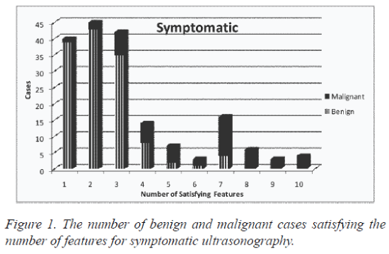
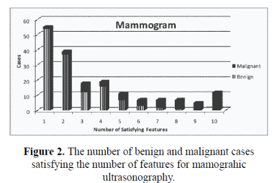
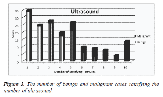
The design was made to accurately predict the output by generating counts and probability. The features from all the three modalities were extracted. The attributes were given a specified domain number along with an identification number. The modalities of Symptomatic, Mammographic and combined Ultrasonography & Elastography were given domain numbers as two, three and four respectively with integer values from ‘1’ to ‘10’ with their corresponding satisfying features from trained database. The number of benign and malignant cases satisfying the number of features for symptomatic, mammographic and ultrasound are given in figure 1, figure 2 and figure 3, respectively. The fifth attribute number is given for the decision of the class with domain number as ‘3’ and ‘6’ for benign and malignant respectively.
The first classifier works on the principle of linear or nonlinear classifier which separates a set of cases into their corresponding groups (benign and malignant) with a segment [19-21]. The classifier categorized the set of cases with a decision into two class membership function. The classification task is by construction of hyper planes in a multi-dimensional space by handling multiple continuous and categorical variables having either ‘0’ or ‘1’. A hyper plane was constructed using the number of satisfying features as well as the BI-RADS category for indicating benign or malignant as its axes.
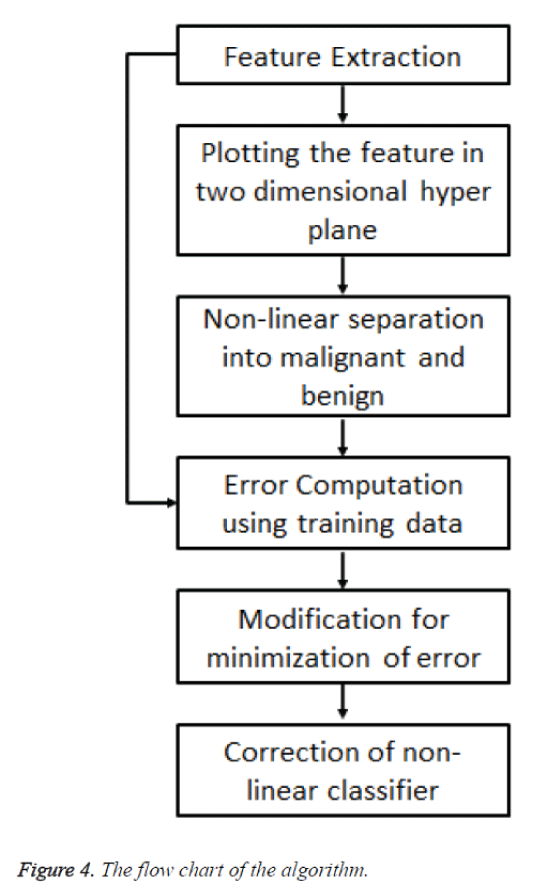
A non-linear classifier is used for the separation in the hyper plane. The error function is calculated and is minimized over multiple iterations using the training data. A non-linear kernel is preferred for this application requirement for minimizing the error function by sequential optimization. The boundary on the right side or beyond the boundary is for all cases that are benign and to left or within the boundary is for all cases that are malignant. The flow chart of the algorithm used is given in figure 4.
The second classifier is based on optimization and uses high dimensional inputs performing more sophisticated classification methods. On application of training dataset, the optimization of classifiers was implemented by determining the probability of associating certain classes at particular events given the instances of the predictor variables.
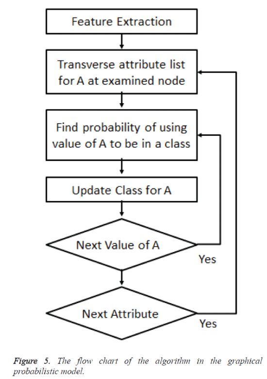
The cases were classified as benign or malignant and the probability of benign or malignant is found based on the number of benign or malignant cases. A likelihood of benign is based on the probability of benign case in the vicinity of the case with reference to all the benign cases. Same is the probability with respect to the malignant cases. When there were more benign cases than malignant it was logically believed that the new case was twice likely having membership benign rather than malignant. Classification was by prior probability. The flow chart of the algorithm is given in figure 5. The nodes are the variables in the graphical probabilistic model.
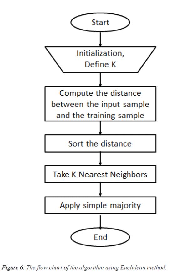
The optimization of posterior probability of the third classifier is done by combining both prior and the likelihood. Using the third classifier the model for classification involved the task of classifying a new case by instance based analysis which was the query point from a number of recognized cases. The task was classifying the decision of the query point from a selected number in its nearest neighbors. Considering set of points which were benign a curve was drawn from the relationship between the independent and dependent variable. From the set of benign cases the method was used to predict the outcome which was the new case from the set of benign. A distance metric was defined for measuring the distance between the query point and cases from the sample for the predictions using Euclidean method. The flow chart of the algorithm is given in figure 6.
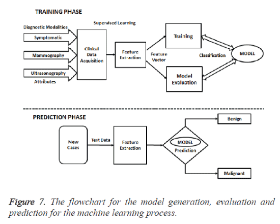
The training phase of the model was evaluated with Biopsy which is considered as the gold standard diagnostic procedure. The flowchart for the model generation, evaluation and prediction for the machine learning process is given in figure 7. Thus the class distribution table had 132 benign cases (73.3%) and 48 malignant cases (26.7%) out of the 180 instances. The ten features from modalities with ‘present’ or ‘not present’ is elaborated in table 3. Mammographic, Ultrasound and Biopsy findings of the study population during the training and testing phases is given in table 4.
| Symptomatic | Mammography | Ultrasonography | |||||||
|---|---|---|---|---|---|---|---|---|---|
| Features | B | M | Total | B | M | Total | B | M | Total |
| 1 | 39 | 1 | 40 | 54 | 1 | 55 | 34 | 1 | 35 |
| 2 | 43 | 2 | 45 | 37 | 2 | 39 | 24 | 1 | 25 |
| 3 | 35 | 7 | 42 | 12 | 6 | 18 | 26 | 2 | 28 |
| 4 | 8 | 6 | 14 | 16 | 3 | 19 | 17 | 3 | 20 |
| 5 | 2 | 5 | 7 | 7 | 4 | 11 | 21 | 6 | 27 |
| 6 | 1 | 2 | 3 | 3 | 4 | 7 | 6 | 4 | 10 |
| 7 | 4 | 12 | 16 | 2 | 5 | 7 | 3 | 6 | 9 |
| 8 | 0 | 6 | 6 | 1 | 6 | 7 | 1 | 7 | 8 |
| 9 | 0 | 3 | 3 | 0 | 5 | 5 | 0 | 4 | 4 |
| 10 | 0 | 4 | 4 | 0 | 12 | 12 | 0 | 14 | 14 |
| Total | 132 | 48 | 180 | 132 | 48 | 180 | 132 | 48 | 180 |
| Mean | 2.32 | 5.96 | 3.29 | 2.30 | 6.81 | 3.50 | 3.02 | 7.27 | 4.15 |
| SD | 1.32 | 2.42 | 2.33 | 1.55 | 2.77 | 2.79 | 1.72 | 2.50 | 2.71 |
| Mode | 2 | 7 | 2 | 1 | 10 | 1 | 1 | 10 | 1 |
| Median | 2 | 7 | 3 | 2 | 7 | 2 | 3 | 8 | 4 |
| 95% CImean | 1.377 3.263 |
4.230 7.690 |
1.625 4.955 |
1.192 3.408 |
4.830 8.790 |
1.506 5.494 |
1.791 4.249 |
5.483 9.057 |
2.213 6.087 |
SD, standard deviation; T-value, hypothetic test value; CI, confidence interval; B,
Benign; M, Malignant
Table 3. Training dataset interpretation for three modalities.
| Parameters | Training Phase | Testing Phase | ||
|---|---|---|---|---|
| Benign | Malignant | Benign | Malignant | |
| Mammographic Breast density | ||||
| Entire fatty Grade 1 | 18 | 9 | 44 | 8 |
| Scattered areaGrade 2 | 32 | 17 | 41 | 2 |
| HeterogeneouslyGrade 3 | 37 | 13 | 35 | 6 |
| Extremely DenseGrade 4 | 45 | 9 | 56 | 18 |
| Size of breast masses(cm) | 1.96±0.4 | 1.85±0.6 | 1.96±0.7 | 1.89 ±0.2 |
| BI-RADS Category (Suspicion for malignancy) |
||||
| (1% )Score 3 | 5 | 3 | ||
| (13%)Score4a | 8 | 7 | ||
| (36%) Score4b | 8 | 4 | ||
| (79%) Score4c | 11 | 9 | ||
| (95%)score 5 | 16 | 11 | ||
| Benign (Biopsy result) | ||||
| Fibrocystic change | 45 | 47 | ||
| Fibro adenoma | 26 | 34 | ||
| Papilloma | 17 | 27 | ||
| Adenosis | 13 | 22 | ||
| Ductal epithelial hyperplasia | 8 | 10 | ||
| Columnar cell change | 6 | 12 | ||
| Benign phyllodestumor | 3 | 8 | ||
| Lobular carcinoma in situ | 1 | 3 | ||
| Radial scar | 7 | 6 | ||
| Chronic granulomatous inflammation | 4 | 2 | ||
| Lipoma | 2 | 1 | ||
| Fat necrosis | 6 | 4 | ||
| Malignant (Biopsy) | ||||
| Invasive ductal carcinoma | 24 | 19 | ||
| Invasive lobular carcinoma | 4 | 2 | ||
| Tubular carcinoma | 1 | 1 | ||
| Ductal carcinoma in situ | 11 | 8 | ||
| Inflamatory carcinoma | 5 | 3 | ||
| Medullary carcinoma | 1 | 0 | ||
| Mucinous (or colloid) carcinoma | 2 | 1 | ||
Table 4. Mammographic, Ultrasound and Biopsy findings of the study population during the training and testing phases.
Results
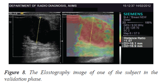
The comparison of mean (T-test) with 95% confidence interval level for Symptomatic was 1.625 to 4.955, Mammographic was 1.506 to 5.494 and ultrasound Elastography imaging was 2.213 to 6.087 with p<0.0001 for all the three classifiers. The Elastography image of one of the subject in the validation phase is given in figure 8. A total of 210 cases were used in testing the data and compared with the Biopsy data. The statistical analysis using the dataset taken in testing phase is represented in table 3.
True positive, true negative, false positive and false negative values from confusion matrix were used for analysis of statistical data. The statistical analysis was evaluated using the classification models for its specificity, sensitivity, accuracy, Fscore, Youden's index and the ROC curve [22]. Statistically significance was considered for a two-tailed P value <0.05 [23]. Less false positive cases improved the diagnostic efficiency. The feature selection for sparse representation based classification algorithm from mammographic gray scale information were also analyzed and compared [24]. The error rate was 4.29%, 15.71% and 8.57% in order for all the three classifiers shown in table 5.
| Parameters | Classifier-1 | Classifier-2 | Classifier-3 |
|---|---|---|---|
| True positive | 31 | 22 | 28 |
| False positive | 6 | 21 | 12 |
| False negative | 3 | 12 | 6 |
| True negative | 170 | 155 | 164 |
| Sensitivity | 0.912 | 0.647 | 0.824 |
| Specificity | 0.966 | 0.881 | 0.932 |
| Precision | 0.838 | 0.512 | 0.700 |
| Accuracy | 0.957 | 0.843 | 0.914 |
| Negative predictive value | 0.983 | 0.928 | 0.965 |
| Κappa-value | 0.791 | 0.650 | 0.738 |
| F-Score | 0.873 | 0.571 | 0.757 |
| G-Score | 0.874 | 0.575 | 0.759 |
| Informedness | 0.820 | 0.440 | 0.665 |
| Markedness | 0.878 | 0.528 | 0.755 |
| Pearsons coefficient | 0.849 | 0.482 | 0.709 |
| p-value | <0.0001 | <0.0001 | <0.0001 |
| Area Under the Curve | 0.939 | 0.764 | 0.878 |
| Youden Index | 0.878 | 0.528 | 0.755 |
Table 5. Statistical analysis of the three individual classifiers
Discussion
The typical diagnostic scenario of the three classifiers are discused based on a malignant and a benign case. They were evaluated as follows:
Case 1: Analysis on a female patient of 34 years
External symptoms: Mastalgia Breast lump felt near left axilla, fluid Discharge in Nipple.
Mammography: Lobulated hypoechoic vascularized mass and oval in shape
Ultrasonography: Oval hypoechoic mass of size 1.87cm X 1.58cm at 4o clock position at LOQ indistinguishable from fibroadenoma, suspicious and was categorized to BIRADS 4. Machine learning: The three classifiers showed the probabilities of 95%, 87% and 93% benign respectively. Biopsy showed Fibrous tissues with no signs of malignancy.
Case 2: Evaluation on a 56 year old woman
Symptoms: sticky secretion in nipple, Nipple retraction on right breast, painful but not progressive.
Mammography: Lobulated solid mass 1.06cm, 0.56cm with multi-centric ductal expansion to different quadrants of the right breast.
Ultrasonography: Nodes with cortical thickening and multiple lesions< 2 cm in different segments of the breast.
Malignancy was assigned from the probabilities of 98%, 91% and 92% for the classifiers. Biopsy proved Infiltrating Ductal Carcinoma.
The mammographic imaging features represent data relevant to breast cancer diagnosis, [25,26]. Mostly inconclusive and suspicious cases are followed up with ultrasound after mammogram, [27]. Patients with palpable masses used breast ultrasound examination and those with bulging masses and/or deformed breast outlines used mammography as the first line imaging examination, [28]. The high accuracy achieved in the diagnostic prediction using Symptomatic, Mammographic and Ultrasound Elastography datasets is a positive step towards avoiding biopsy which was considered as the gold standard. The efficiency of the classifiers was more than 95% with classifier-1 proving to be the best. Hence use of classifier-1 is recommended.
References
- Guo L, Rivero D, Dorado J, Munteanu CR, Pazos A. Automatic feature extraction using genetic programming: An application to epileptic EEG classification. Expert Systems with Applications 2011;38:10425-10436.
- Abrahamsson L, Czene K, Hall P, Humphreys K. Breast cancer tumour growth modelling for studying the association of body size with tumour growth rate and symptomatic detection using case-control data. Breast Cancer Res 2014;17:1-11.
- Yang H, Huang K, King I, Lyu MR. Maximum margin semi-supervised learning with irrelevant data. Neural Networks. 2015;70:90-102.
- Eshlaghy AT, Poorebrahimi A, Ebrahimi M, Razavi AR, Ahmad LG. Using three machine learning techniques for predicting breast cancer recurrence. J Health Med Inform 2013;4:124.
- Casti P, Mencattini A, Salmeri M, Rangayyan RM. Analysis of Structural Similarity in Mammograms for Detection of Bilateral Asymmetry. Medical Imaging, IEEE Transactions on 2015;34:662-671.
- Ramos-Pollán R, Guevara-López MA, Suárez-Ortega C, Díaz-Herrero G, Franco-Valiente JM, Rubio-del-Solar M, et al. Discovering mammography-based machine learning classifiers for breast cancer diagnosis. J Med Syst 2012;36:2259-2269.
- Sadigh G, Carlos RC, Neal CH, Dwamena BA. Accuracy of quantitative ultrasound elastography for differentiation of malignant and benign breast abnormalities: a meta-analysis. Breast Cancer Res Treat 2012;134:923-931.
- Raj JJR, Anand S. Efficient analysis and evaluation of elasticity of breast tumours using ultrasound in Indian women. International Journal of Biomedical Engineering and Technology 2015;18:227-239.
- Liu X-J, Zhu Y, Liu P-F, Xu Y-L. Elastography for Breast Cancer Diagnosis: a Useful Tool for Small and BI-RADS 4 Lesions. Asian Pacific journal of cancer prevention: APJCP 2013;15:10739-10743.
- Carlsen J, Ewertsen C, Sletting S, Vejborg I, Schafer FK, Cosgrove D, et al. Ultrasound Elastography in Breast Cancer Diagnosis. Ultraschall Med 2015.
- Cheng H, Shan J, Ju W, Guo Y, Zhang L. Automated breast cancer detection and classification using ultrasound images: A survey. Pattern Recognition. 2010;43:299-317.
- Sato RC, Sato GTK. Probabilistic graphic models applied to identification of diseases. Einstein (São Paulo) 2015;13:330-333.
- Maldonado S, Weber R, Basak J. Simultaneous feature selection and classification using kernel-penalized support vector machines. Information Sciences. 2011;181:115-128.
- Chalmers E, Mizianty M, Parent E, Yuan Y, Lou E. Toward maximum-predictive-value classification. Pattern Recognition. 2014;47:3949-3958.
- Beck J, Urnovitz HB, Mitchell WM, Schütz E. Next generation sequencing of serum circulating nucleic acids from patients with invasive ductal breast cancer reveals differences to healthy and nonmalignant controls. Mol Cancer Res 2010;8:335-342.
- Hsieh S-L, Hsieh S-H, Cheng P-H, Chen C-H, Hsu K-P, Lee I-S, et al. Design ensemble machine learning model for breast cancer diagnosis. J Med Syst 2012;36:2841-2847.
- Banik S, Rangayyan RM, Desautels JL. Detection of architectural distortion in prior mammograms. Medical Imaging, IEEE Transactions on2011;30:279-294.
- Waske B, van der Linden S, Benediktsson JA, Rabe A, Hostert P. Sensitivity of support vector machines to random feature selection in classification of hyperspectral data. Geoscience and Remote Sensing, IEEE Transactions on2010;48:2880-2889.
- Castillo E, Peteiro-Barral D, Berdiñas BG, Fontenla-Romero O. Distributed One-Class Support Vector Machine. Int J Neural Syst. 2015;25:1550029.
- Datta S, Das S. Near-Bayesian Support Vector Machines for imbalanced data classification with equal or unequal misclassification costs. Neural Networks 2015;70:39-52.
- Nguyen MH, De la Torre F. Optimal feature selection for support vector machines. Pattern recognition. 2010;43:584-591.
- Mert A, Kılıç N, Bilgili E, Akan A. Breast Cancer Detection with Reduced Feature Set. Comput Math Methods Med 2015.
- Lin Y, Liu F, Fan Y, Qian X, Lang R, Gu F, et al. Both high expression of pyruvate kinase M2 and vascular endothelial growth factor-C predicts poorer prognosis in human breast cancer. Int J ClinExpPathol 2015;8:8028.
- Kim DH, Lee SH, Ro YM. Mass type-specific sparse representation for mass classification in computer-aided detection on mammograms. Biomedical engineering online 2013;12:S3.
- Liu J, Wu Y, Ong I, Page D, Peissig P, McCarty C, et al. Leveraging Interaction between Genetic Variants and Mammographic Findings for Personalized Breast Cancer Diagnosis. AMIA Summits on Translational Science Proceedings. 2015;2015:107.
- Ergin S, Kilinc O. A new feature extraction framework based on wavelets for breast cancer diagnosis. ComputBiol Med 2014;51:171-182.
- Mainiero MB, Lourenco AP, Barke LD, Argus AD, Bailey L, Carkaci S, et al. ACR Appropriateness Criteria Evaluation of the Symptomatic Male Breast. J Am CollRadiol 2015.
- Makanjuola D, Alkushi A, Alzaid M, Abukhair O, Al Tahan F, Alhadab A. Breast cancer in women younger than 30 years: prevalence rate and imaging findings in a symptomatic population. The Pan African medical journal 2014;19.
